Buried in the supplement of a recent paper is a variant of this figure that I’m rather proud of:
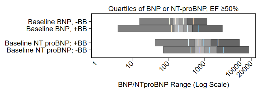
It shows the distribution of quartiles of BNP and NT proBNP at baseline on a log scale, by use of beta blockers (BB) at baseline. It also shows the midway point of the medians. It’s a nice figure that shows the increase of BNP with beta blocker administration. My colleagues jokingly called it the “Plante Plot” since I have had it included in several drafts of manuscripts, this is just the first one in which it was published.
The code for it is pretty complex and follows. Steps 1-3 pluck out the ranges of the quartiles and their midpoints for each group and saves them as a CSV file. Steps 4-8 render the figure. You may find it more simple to skip Steps 1-3 and manually enter the ranges of the quartiles and their medians into an Excel file and just open up that excel file in Step 4.
Alternatively, I have a do file that automates this a bit. Just type:
do https://www.uvm.edu/~tbplante/plante%20plot%20for%20distribution%20of%20quartiles%20v1_0.do
distplot [xaxis variable] [yaxis group name]
Good luck!
// Step 1: load the database
use "029b1b analytic datset.dta", clear

// Step 2: You need quartiles plus the intermediate points of
// each quartile, which is really 8-iles.
// Step 2a:
// You need the maximum and minimum variables to draw the bounds
// of the bottom and top quartile
// this is by group, here's the first group:
sum baseline_bnp if efstratus50==1 & baselinebb0n1y==0, d
return list // see that r(min) and r(max) are the points needed
// save min and max as macros for 0th bound and 0th bound
local bnp8ile_nobb_0=r(min) // beginning of q1
local bnp8ile_nobb_8=r(max) // end of q4
// Step 2b:
// now get intermediate bounds for the 8-iles
_pctile baseline_bnp  if efstratus50==1  & baselinebb0n1y==0, percentiles(12.5(12.5)87.5) // this gets bounds by 12.5iles
return list // there they are!
local bnp8ile_nobb_1=r(r1) // middle of q1
local bnp8ile_nobb_2=r(r2) // end of q1/beginning of q2
local bnp8ile_nobb_3=r(r3) // middle of q2
local bnp8ile_nobb_4=r(r4) // end of q2/beginning of q3
local bnp8ile_nobb_5=r(r5) // middle of q3
local bnp8ile_nobb_6=r(r6) // end of q3/beginning of q4
local bnp8ile_nobb_7=r(r7) // middle of q4
// now come up with a label to eventually apply to the figure
// don't use commas in this label since we'll save this
// output as a CSV file and commas will screw up the cell
// structure of a CSV (C=comma)
// step 2c:
local label_bnp_nobb="Baseline BNP; -BB"

// now repeat for the other groups
sum baseline_bnp if efstratus50==1 & baselinebb0n1y==1, d
return list
local bnp8ile_bb_0=r(min)
local bnp8ile_bb_8=r(max)
_pctile baseline_bnp  if efstratus50==1  & baselinebb0n1y==1, percentiles(12.5(12.5)87.5)
return list
local bnp8ile_bb_1=r(r1)
local bnp8ile_bb_2=r(r2)
local bnp8ile_bb_3=r(r3)
local bnp8ile_bb_4=r(r4)
local bnp8ile_bb_5=r(r5)
local bnp8ile_bb_6=r(r6)
local bnp8ile_bb_7=r(r7)
local label_bnp_bb="Baseline BNP; +BB"

sum baseline_ntprobnp if efstratus50==1 & baselinebb0n1y==0, d
return list
local ntprobnp8ile_nobb_0=r(min)
local ntprobnp8ile_nobb_8=r(max)
_pctile baseline_ntprobnp  if efstratus50==1  & baselinebb0n1y==0, percentiles(12.5(12.5)87.5)
return list
local ntprobnp8ile_nobb_1=r(r1)
local ntprobnp8ile_nobb_2=r(r2)
local ntprobnp8ile_nobb_3=r(r3)
local ntprobnp8ile_nobb_4=r(r4)
local ntprobnp8ile_nobb_5=r(r5)
local ntprobnp8ile_nobb_6=r(r6)
local ntprobnp8ile_nobb_7=r(r7)
local label_ntprobnp_nobb="Baseline NT proBNP; +BB"

sum baseline_ntprobnp if efstratus50==1 & baselinebb0n1y==1, d
return list
local ntprobnp8ile_bb_0=r(min)
local ntprobnp8ile_bb_8=r(max)
_pctile baseline_ntprobnp  if efstratus50==1  & baselinebb0n1y==1, percentiles(12.5(12.5)87.5)
return list
local ntprobnp8ile_bb_1=r(r1)
local ntprobnp8ile_bb_2=r(r2)
local ntprobnp8ile_bb_3=r(r3)
local ntprobnp8ile_bb_4=r(r4)
local ntprobnp8ile_bb_5=r(r5)
local ntprobnp8ile_bb_6=r(r6)
local ntprobnp8ile_bb_7=r(r7)
local label_ntprobnp_bb="Baseline NT proBNP; -BB"


// Step 3: save this to a csv file that we'll open up right away.
// Note: This code goes out of frame on my blog. copy and paste it
// into a .do file and it'll all appear.
quietly {
capture log close bnp
log using "bnprangefigure.csv", replace text name(bnp)
// this is the row of headers:
noisily di "row,label,eight0,eight1,eight2,eight3,eight4,eight5,eight6,eight7,eight8"
// row 1:
noisily di "1,`label_bnp_nobb',`bnp8ile_nobb_0',`bnp8ile_nobb_1',`bnp8ile_nobb_2',`bnp8ile_nobb_3',`bnp8ile_nobb_4',`bnp8ile_nobb_5',`bnp8ile_nobb_6',`bnp8ile_nobb_7',`bnp8ile_nobb_8'"
// row 2
noisily di "2,`label_bnp_bb',`bnp8ile_bb_0',`bnp8ile_bb_1',`bnp8ile_bb_2',`bnp8ile_bb_3',`bnp8ile_bb_4',`bnp8ile_bb_5',`bnp8ile_bb_6',`bnp8ile_bb_7',`bnp8ile_bb_8'"
// blank row 3:
noisily di "3"
// row 4:
noisily di "4,`label_ntprobnp_nobb',`ntprobnp8ile_nobb_0',`ntprobnp8ile_nobb_1',`ntprobnp8ile_nobb_2',`ntprobnp8ile_nobb_3',`ntprobnp8ile_nobb_4',`ntprobnp8ile_nobb_5',`ntprobnp8ile_nobb_6',`ntprobnp8ile_nobb_7',`ntprobnp8ile_nobb_8'"
// row 5:
noisily di "5,`label_ntprobnp_bb',`ntprobnp8ile_bb_0',`ntprobnp8ile_bb_1',`ntprobnp8ile_bb_2',`ntprobnp8ile_bb_3',`ntprobnp8ile_bb_4',`ntprobnp8ile_bb_5',`ntprobnp8ile_bb_6',`ntprobnp8ile_bb_7',`ntprobnp8ile_bb_8'"
log close bnp
}

// step 4: open CSV file as active database:
import delim using "bnprangefigure.csv", clear
// note, you may opt to skip steps 1-3 and manually compile the
// ranges of each quartile and their median into an excel file.
// Use the -import excel- function to open that file up instead.
// IF YOU SKIP OVER STEPS 1-3, your excel file will need the
/// following columns:
// row - each group, with a blank row 3 to match the figure
// label - title to go to the left of the figure
// eight0 through eight8 - the even numbers are ranges of the
//    quartiles and the odd numbers are the mid-ranges.
//    See my approach in steps 2a-2b on how to get these numbers.

// step 5: steal the labels. note skipping row 3 since it's blank
local label1=label[1]
local label2=label[2]
local label4=label[4] // NO ROW 3!!
local label5=label[5]

// step 6: pluck the intermediate points of each quartile
// which are 8-iles 1, 3, 5 and 7
// and repeat for each row
local bar1row1=eight1[1]
local bar2row1=eight3[1]
local bar3row1=eight5[1]
local bar4row1=eight7[1]

local bar1row2=eight1[2]
local bar2row2=eight3[2]
local bar3row2=eight5[2]
local bar4row2=eight7[2]

// no row 3 in this figure

local bar1row4=eight1[4]
local bar2row4=eight3[4]
local bar3row4=eight5[4]
local bar4row4=eight7[4]

local bar1row5=eight1[5]
local bar2row5=eight3[5]
local bar3row5=eight5[5]
local bar4row5=eight7[5]

// step 7: pick a different scheme than the default stata one
// I like s1mono or s1color
set scheme s1mono

// step 8: complex graph.
// NOTE: RUN THIS SCRIPT FROM THE TOP EVERY TIME because
// stata likes to drop the macros ("local" commands) and
// the things inside of the ticks will be missing if you
// just run starting at the "graph twoway" below
//
// step 8a: rbar the ends of the quartiles, which is:
// 0 to 2, 2 to 4, 4 to 6, and 6 to 8
//
// step 8b: apply the labels
//
// step 8c: place a vertical bar at the midpoints of the
// quartiles, which are at: 1, 3, 5, and 7. A bug in Stata
// is that a centered label (placement(c)) is actually a smidge
// south still, so the rows are offset by 0.13. You'll notice
// the Y label in the text box is row value minus 0.13 (0.87, etc.)
// to account for that.
//
// step 8d: adjust the aspect ratio to get the bar character ("|")
// to fit within the width of the the bar itself.
//

graph twoway /// step 8a:
(rbar eight0 eight2 row , horizontal) ///
(rbar eight2 eight4 row , horizontal) ///
(rbar eight4 eight6 row , horizontal) ///
(rbar eight6 eight8 row , horizontal) ///
, ///
yscale(reverse) ///
xscale(log) ///
t2title("Quartiles of BNP or NT-proBNP, EF ≥50%", justification(center)) ///
xla(1 "1" 10 "10" 100 "100" 1000 "1000" 10000 "10000" 20000 "20000", angle(45)) /// step 8b:
yla(1 "`label1'" 2 "`label2'" 4 "`label4'" 5 "`label5'", angle(horizontal)) ///
ytitle(" ") ///
xtitle("BNP/NTproBNP Range (Log Scale)") ///
legend(off) ///
/// step 8c:
text(0.87 `bar1row1' "|", color(white) placement(c)) ///
text(0.87 `bar2row1' "|", color(white) placement(c)) ///
text(0.87 `bar3row1' "|", color(white) placement(c)) ///
text(0.87 `bar4row1' "|", color(white) placement(c)) ///
///
text(1.87 `bar1row2' "|", color(white) placement(c)) ///
text(1.87 `bar2row2' "|", color(white) placement(c)) ///
text(1.87 `bar3row2' "|", color(white) placement(c)) ///
text(1.87 `bar4row2' "|", color(white) placement(c)) ///
///
text(3.87 `bar1row4' "|", color(white) placement(c)) ///
text(3.87 `bar2row4' "|", color(white) placement(c)) ///
text(3.87 `bar3row4' "|", color(white) placement(c)) ///
text(3.87 `bar4row4' "|", color(white) placement(c)) ///
///
text(4.87 `bar1row5' "|", color(white) placement(c)) ///
text(4.87 `bar2row5' "|", color(white) placement(c)) ///
text(4.87 `bar3row5' "|", color(white) placement(c)) ///
text(4.87 `bar4row5' "|", color(white) placement(c)) ///
/// step 8d:
aspect(0.23)