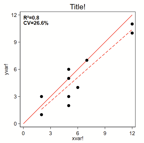
The below code outputs this figure. I grabbed the %CV-from-a-regression code from Mehmet Mehmetoglu’s CV program. (Type –ssc install cv– to grab that one. It’s not needed for below.) By the way, you might also be interested in how to make a related Bland-Altman plot here.

Here’s the code:

// note this uses local macros so you need to run this entire thing
// top to bottom in a do file, not line by line. 
//
// Step 1: input some fake data:
clear all

input id y x
1 2 5
2 3 5
3 6 5
4 7 7
5 3 2
6 10 12
7 1 2
8 11 12
9 4 6
10 5 5
end

// Step 2a: Grab the R2 from a regresssion
regress y x
local rsq = e(r2)
// Step 2b, from the same regression, calculate the percent CV
local  rmse= e(rmse)
local depvar = e(depvar)
sum `depvar' if e(sample), meanonly
local depvarmean = r(mean)
local cv = `rmse'/`depvarmean'*100

// Step 3: graph!
set scheme s1mono // I like this scheme

twoway ///
/// Line of unity, you'll need to tweak the range for your data:
(function y=x , range(0 12) lcolor(red) lpattern(solid) lwidth(medium)) ///
/// line of fit:
(lfit y x,  lcolor(red) lpattern(dash) lwidth(medium)) ///
/// Scatter plot dots:
(scatter y x, msymbol(O) msize(medium) mcolor(black)) ///
, ///
aspect(1) /// force output to be square
/// here's the text box with R2 and CV,
/// you'll need to tweak the first two numbers so the y,x
/// coordinates drop the text where you want it
text(12 0 "{bf:R²=`:di %3.1f `=`rsq'''}" "{bf:CV=`:di %4.1f `=`cv'''%}", placement(se) justification(left)) /// 
legend(off) /// Shut off the legend
yla(0(3)12, angle(0)) /// you'll need to tweak range for your data
xla(0(3)12) /// you'll need to tweak range for your data
ytitle("Y!") ///
xtitle("X!") ///
title("Title!")