Note in 2023: We are using R and not Stata this summer so this post doesn’t apply to this year’s projects.

Stata is a popular commercial statistical software package that was first released 30+ years ago. It has some really nice features, loads of top-rate documentation, a very active community, and approachable syntax. For beginners, I think it’s the simplest to learn.

Learning how to use Stata

Stata has really, really, really good documentation.

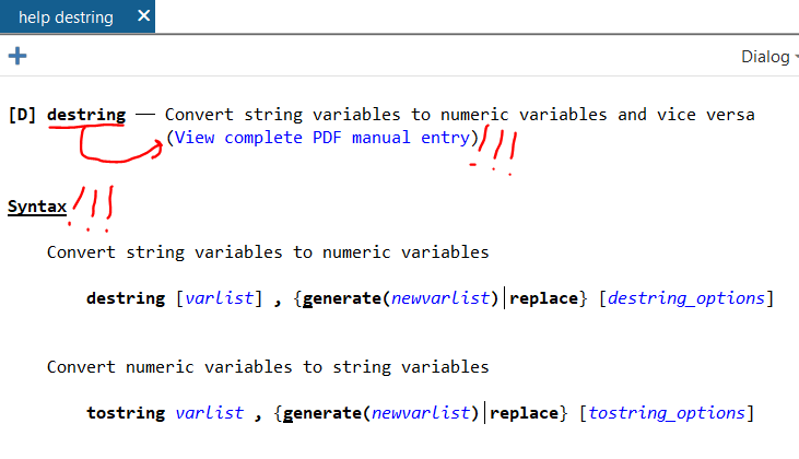
The documentation is outstanding. Let’s say that you want to learn how to use the –destring– command. In the command line (1a under “Stata’s Interface” below), type:

help destring

…and up will pop a focused help file. There’s the “View complete PDF manual entry” option that has EXTENSIVE documentation of the command. (Note: This file seems to only work well with Adobe PDF reader, not alternative PDF readers like Sumatra). If the focused help file isn’t sufficient to answer your questions, try the complete PDF manual.

The focused help file has multiple parts, but the syntax example is gold. Further down you’ll see example uses of the command.

Web searches will find even more answers

Odds are that someone has already hit the same problem you have in using Stata. Queries in your favorite search engine are likely to find answers on the Statalist archive or UCLA’s excellent website.

You can install Stata programs that other users have written

There are MANY MANY MANY user-written programs out there that can be installed and used in your code. You only need to install them once. Most are on BU’s repository called SSC. I use the table1_mc program extensively (it makes pretty table 1s, you can read about it here). To install table1_mc from SSC, you type:

ssc install table1_mc

…and Stata will download it and install it for you. It’s ready to use when it finishes installing. And, there’s no need to re-install it, it will load each time you start Stata.

Quirks of Stata

Stata only works with rectangular datasets

Think of a rectangular dataset as a single spreadsheet in Excel. It has vertical columns and horizontal rows. There’s no data on a Z axis coming out of the computer at your face.

A rectangular dataset is the only type that Stata works with. Other statistical software like R or Python can handle many more complex data structures. For learners, forcing data to fit within a rectangular dataset is a huge advantage in my mind since that structure is intuitive, and you can always browse your data with the built-in data browser (see 3c under Stata’s Interface, below).

Stata only works with one dataset at a time*

One dataset in Stata is akin to one spreadsheet in a workbook in Excel. In Excel, you can have multiple spreadsheets in one .xlsx workbook file, with each spreadsheet appearing on a different tab at the bottom. All spreadsheets are in the memory at the same time. You can do math across spreadsheets in a workbook in excel, summarize costs in one column in spreadsheet A and have the result appear in one cell on spreadsheet B. In Stata, you can only have one spreadsheet (here, dataset) open at a time.* Because of this, Stata users spend a good deal of time merging and appending multiple datasets to make a single dataset that has all of the necessary variables in the best format from the get-go.

A big problem historically with Stata was that datasets are loaded in the RAM, and big datasets would be too big for conventional computers. That’s not an issue anymore since even cheap computers have several gigabytes of RAM.

*This isn’t true anymore. Starting in version 16, Stata can actually now have multiple datasets in memory, each stored in its own frame. These frames can be very useful in certain scenarios, but for our purposes, we are going to pretend that you can have just one dataset open at a time.

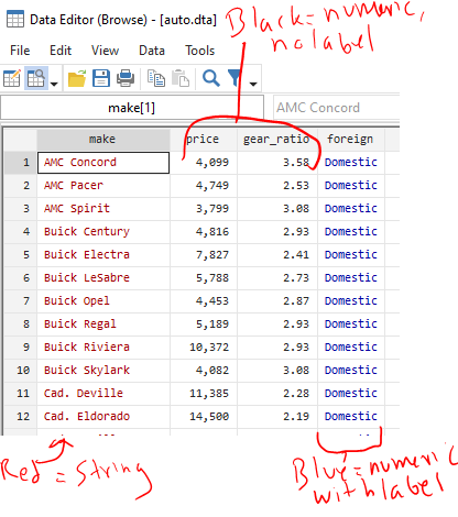
Data are either string or numeric. Their color changes in the data browser

Strings are basically text that are thought to be words and not numbers. But sometimes a dataset will be imported wrong and things that are actually numbers (“1.5”, “2.5” in different rows of the same column) will be imported and considered to be strings and not numbers. This might be because they were imported incorrectly. This might be that later down in the list there is a word in a different cell (“1.5”, “2.5”, “Specimen error”). If any row of a variable contains something that isn’t a number, Stata makes the entire column, and with it the variable, a string.

IMPORTANT: When viewing strings in the data browser (3c under “Stata’s Interface” below), they appear in RED text. When specifying strings in commands, you need to enclose them in quotations (eg count if name==”Old”). Missing strings are two quotes with nothing in between them (eg count if name==””).

In order to do math, you need to have things be numbers. There are several different numerical formats that you can read about here. If something is an integer (nothing after the decimal), it can be byte, int, and long. If something has a decimal point, it’s float or double. Stata does a nice job selecting which numerical format your data should be in, so you probably don’t need to think much about the difference between byte, int, long, float, or double again.

IMPORTANT: When viewing numeric variables in the data browser, they appear in BLACK text (or BLUE if they have a label applied). When specifying strings in commands, no quotations are needed (eg count if quartile==1). Missing strings are periods (eg count if quartile==.), and a period is positive infinity (a missing value is bigger than a value of one billion).

To convert from a string to a numerical value (change the “1” to a 1), you use the –destring– command. You might need to include the force and replace options, but read up on those by typing –help destring–.

To convert from a numerical value to a string (change the “1” to a 1), use the –tostring– command. Note that missing numerical values will go from a dot to a dot in quotations (. becomes “.”), which is not the same as a missing value for a string, which is just empty quotations (“”). It’s a good idea to follow up a –tostring– command with a command that replaces “.” values with “” values.

Stata’s output is only 255 characters wide, max

The output window of Stata will print (“display”) the inputted command and results from that command. It will clip the output at up to 255 characters, and insert a line break to the next row. You can specify:

set linesize 255

…so that the output is always 255 characters wide. Otherwise, it’ll adjust the output to match how wide your output window is.

The working directory is your “documents folder” unless you manually set the working directory with the cd command or open up Stata by double clicking on a .do file in Windows explorer

The working directory is where Stata is working from. If you save a dataset with the –save– command, it’ll save it in the working directory unless you specify all of the files from the C: drive on. If you double click on the Stata icon to open it up in Windows and type the present working directory command to see where it’s working from (that’s –pwd–), it’ll print out:

. pwd 
C:\Users\USERNAME\Documents

So, if you type:

save "dataset.dta", replace

…it’ll save dataset.dta in C:\Users\USERNAME\Documents

Let’s say that you really want to be working in your OneDrive folder because that’s secure and backed up and your Documents folder isn’t. The directory for your desired folder is:

C:\Users\USERNAME\OneDrive\Research project\Analysis

In order to save your file there, you’d type:

save "C:\Users\USERNAME\OneDrive\Research project\Analysis\dataset.dta", replace

Note that there’s a space in the Research project folder name so the directory needs to be in quotations. If there was no space anywhere in the directory, you could omit the quotations. I’m including quotations everywhere here because it’s good practice.

One option is to change your working directory to the OneDrive folder. You use the –cd– command to do that then any save command will automatically save in that folder:

cd "C:\Users\USERNAME\OneDrive\Research project\Analysis\"
save "dataset.dta", replace

Alternatively, you can save your project’s Do file in the “C:\Users\USERNAME\OneDrive\Research project\Analysis\” folder. Rather than opening Stata by clicking on the icon, find the Do file in your OneDrive folder in Windows Explorer and double click on it. It’ll open Stata AND set that folder as the working directory!! For a new project, this means opening Stata by clicking on its icon, opening a blank do file, saving that do file in your OneDrive folder, closing the Do File Editor and Stata, then reopening stata by double clicking on your blank do file in Windows Explorer.

Stata is most effectively used with with command-line input, specifically through the Do File Editor. There is a graphical user interface that can be handy.

I think that everything in Stata should be completed through Do files. These are text files with sequential lines of codes that make Stata perform commands in order.

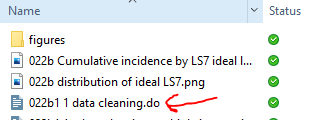
I strongly, strongly, strongly recommend having a set number of do files, the first (“01 cleanup.do”) will merge original data files, generate new variables, print out your inclusion flow diagram, and save your analytical dataset (“analytical.dta”). The rest of the files all do just one thing, like make a table or render a figure. All other files except for the first (“01 cleanup.do”) will first (a) open your analytical dataset (“analytical.dta”) then (b) run some sort of stats without modifying the analytical dataset. I also have one last miscellaneous one for random things that you might need from the text (“99 misc things for text.do”), like estimating median and IQR follow up or some one-off t-tests. If you realize in a later do file (say “02 table 1.do”) that you need to generate a new variable or merge in another raw dataset that you didn’t realize that you needed when you first built your “analytical.dta” dataset, resist the impulse to make new variables in your “02 table 1.do” file and instead go back and rework your “01 cleanup.do” file to generate that variable or merge in another raw dataset. Then, rerun your “01 cleanup.do” file it so it overwrites your “analytical.dta” dataset, and then go back and continue working on your “02 table 1.do” file.

So, your do file directory might look like this:

• 01 cleanup.do – (a) Merge original data files, (b) generate new variables, (c) print out an inclusion flow diagram and (d) also builds your “analytical.dta” analytical dataset that all other do files will use.
• 02 table 1.do – Opens “analytical.dta” then uses table1_mc or something similar to make a table 1.
• 03 histogram of exposure.do – Opens “analytical.dta” then uses the –histogram– command to draw a distribution of your exposure.
• 04 event table.do – Opens “analytical.dta” then uses some sum commands to print out the # of events by group of interest.
• 05 regressions.do – Opens “analytical.dta” then runs your regressions.
• 06 spline.do – Opens “analytical.dta” then runs some code to make restricted cubic splines.
• 99 misc things for text.do – Opens “analytical.dta” then runs one-off code for random details that you might need for the text (e.g., median and IQR follow-up).

GUI in Stata

There is a graphical user interface (GUI) with clickable menus. You can click through commands and it’ll generate the code and run the command of interest, and these can be handy for stealing syntax to run an annoying command. The command from the GUI will appear in the Command History (1c below) and you can right click and copy/paste it into your do file.

I find –import excel– to be frustrating and use the GUI probably 90% of the time to generate that command then copy/paste the syntax into my do file.

You’ll be much better off if you use a do file for nearly everything. Try to minimize the use of the GUI.

Stata won’t let you close a dataset in the memory or overwrite an existing dataset without some effort

The –use– command will open up a dataset in the memory. If you don’t have a dataset opened yet, this will open one:

use dataset.dta

Remember that Stata can only have one dataset opened at a time, so any time you open one when you already have a different dataset opened in memory, Stata will need to drop the open dataset. If you spent a lot of time on the open dataset creating new variables or merging with other datasets, closing it will make you lose all of your work unless you have also saved it. Stata doesn’t want you to make this mistake so if you already have a dataset opened and you type in the above command, Stata will say “No” and you won’t be opening the new dataset.

Instead, you need to put “–, clear–” at the end of the command, like this:

use dataset.dta, clear

And now Stata will drop whatever you have open. It’s really just a nice check to keep you from discarding your work accidentally.

Similarly, if you are trying to save a dataset with the –save– command into an empty folder, you just need to type:

save newdataset.dta

…and Stata will save it no problem. HOWEVER if you are trying to overwrite an existing dataset with that same name, Stata will say “No” and you won’t be saving your dataset today. This is another check. instead, you just need to use “–, replace–” to overwrite. Example:

save newdataset.dta, replace

Stata’s interface

Here’s a quick overview of the Stata interface in Windows.

1. Ways to input and interact with commands:
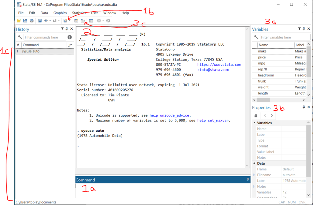
   1a. Command line – This is where you type command by command. Unless you are just poking around in your data, you should avoid using this. Anything that you want to reproduce in your analysis should be done in the Do file editor.
   1b. Open Do file editor button – The Do File Editor is the most important part of Stata in my opinion. A do file is a long text file saving command after command. This is where you should do all of your analytical work.
   1c. Command history – If you use the command line or GUI to make a command, it’ll be saved here. You can right click on old commands and copy/paste them into your do file.
2. Output window – Your command will appear here with a preceding dot (“. sysuse auto” means that I had previously typed in “sysuse auto”). The output from your do file or command will appear immediately below.
3. Ways to interact with data
   3a. Variable list – This is a list of variables in the open dataset. You can double click on them and the variable name will be copied to the command line. You can ctrl+click and select multiple and then copy them to the clipboard. This is quite handy.
   3b. Variable and dataset properties – This will let you see details about a selected variable in the variable list and the current dataset in memory.
   3c. Data browser – You can also pop this open with the –bro– command. this views all data in a spreadsheet format that looks like Excel.