Stata is great because of its intuitive syntax, reasonable learning curve, and dependable implementation. There’s some cutting edge functionality and graphical tools in R that are missing in Stata. I came across the Rcall package that allows Stata to interface with R and use some of these advanced features. (Note: this worked for me as far back as Stata 16. I have no reason to think that this wouldn’t work with Stata 13 or newer.)
Below details:
- How to get set up with Rcall
- Example 1: How to make figures with the ‘ggplot2’ and ‘ggstatsplot’ R packages
- Example 2: How to estimate the Charlson comorbidity index or Elixhauser comorbidity score with the ‘comorbidity’ R package
- Example 3: Estimating race by last name and sex by first name with the ‘predictrace’ R package
- Example 4: Making a heatplot with lattice/levelplot
Installation of R, R packages, and Rcall (you only need to do this once)
Download and install R. (Note: If you have problems this working with an old version of R, such with outdated packages, uninstall R and then also delete the folder that includes the local install packages. On my Windows PC, it was at: C:\Users\[username]\AppData\Local\R\win-library\4.5\. The “Local” folder is hidden, so in Windows Explorer allow hidden folders to be seen under options –> view –> hidden files and folders). Open R and install the readstata13 package, which is required to install Rcall. While you’re at it, install ggplot2 and ggstatsplot. Note: ggplot2 is included in the excellent multi-package collection called Tidyverse. We are going to install Tidyverse instead of ggplot2 alone. Tidyverse also installs several other packages useful in data science that you might need later. This includes dplyr, tidyr, readr, purrr, tibble, stringr, forcats, import, wrangle, program, and model. I have also gotten an error saying “‘Rcpp_precious_remove’ not provided by package ‘Rcpp'”, which was fixed by installing Rcpp, so install that too.
In R, type:
install.packages("readstata13")
install.packages("tidyverse")
install.packages("ggstatsplot")
install.packages("Rcpp")
It’ll prompt you to set up an install directory and choose your mirror/repository. Just pick one geographically close to you. After these finish installing, you can close R.
Rcall’s installation is within Stata (as usual for Stata programs) but originates from Github, not the usual SSC install. You need to install a separate package to allow you to install things from Github in Stata. From the Stata command line, type:
net install github, from("https://haghish.github.io/github/")Now install Rcall itself from the Stata command line:
github install haghish/rcall, stableIf all goes well, it should install!
Edit: In July 2024, there seems to be a problem with the installation. If you get an error saying “github package was not found” and “please update your GitHub package”, you might try to install an older version of rcall than the current version (which is 3.1.0 in 7/2024) as such:
github install haghish/rcall, version(3.0.7)Using Rcall
You should read details on the Rcall help file (type –help rcall– in Stata) for an overview. Also read the Rcall overview on Github. In brief, you can send datasets from Stata to R using –rcall st.data()–. You can kick things back to stata with –st.load(name of R frame)–. –rcall clear– reboots R as a new instance.
There are four modes for using Rcall: vanilla, sync, interactive, and console. For our purposes, we are going to focus on the interactive mode since this allows you to manipulate R from within a do file.
Example 1: Make a figure in ggplot2 using Stata and Rcall
Here’s some demo code to make a figure with ggplot2, which is the standard for figures in R. There’s a handy cheat sheet here. This intro page is quite helpful. This overview is excellent. Check out the demo figures from this page as well. If your ggplot command extends across multiple lines, make sure to end each line (except the final line) with the three forward slash (“///”) line break notation that is used by Stata.
// load sysuse auto dataset
sysuse auto, clear
// set up rcall, clean session and load necessary packages
rcall clear // starts with a new instance of R
rcall: library(ggplot2) // load the ggplot2 library
// move Stata's auto dataset over to R and prove it's there.
rcall: data<- st.data() // move auto dataset to r
rcall: names(data) // prove that you can see the variables.
rcall: head(data, n=10) // now look at the first 10 rows of the data in R
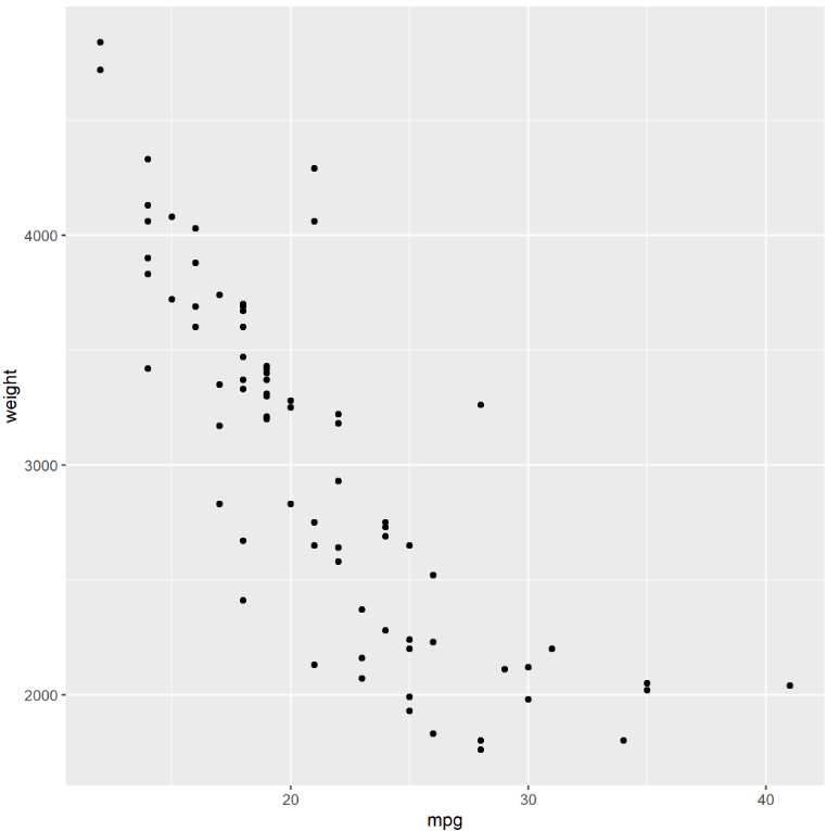
// now make a scatterplot with ggplot2, note the three slashes for line break
rcall: e<- ggplot(data, aes(x=mpg, y=weight)) + ///
geom_point()
rcall: ggsave("ggtest.png", plot=e)
// figure out where that PNG is saved:
rcall: getwd()Note: rather than using the three forward slashes, you can also change the delimiter to a semicolon, like the following. Just remember to change it back to normal (“cr”). Here’s an equivalent to above with semicolon delimiters. Note that the ggplot bit that spreads across two lines no longer has any slashes. This looks a bit more like “true R code”.
sysuse auto, clear
#delimit ;
rcall clear ;
rcall: library(ggplot2) ;
rcall: data<- st.data() ;
rcall: names(data) ;
rcall: head(data, n=10) ;
rcall: e<- ggplot(data, aes(x=mpg, y=weight)) +
       geom_point() ;
rcall: ggsave("ggtest.png", plot=e) ;
rcall: getwd() ;
#delimit cr
Here’s what it made! It was saved in my Documents folder, but check the output above to see where you working directory is.
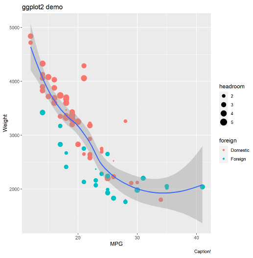
You can get much more complex with the figure, like specifying colors by foreign status, specifying dot size by headroom size, adding a loess curve with 95% CI, and adding some labels. You can swap out the “rcall: e <- ggplot(…)" bit above for the following. Remember to end every non-final line with the three forward slashes.
rcall: e<- ggplot(data, aes(x=mpg, y=weight)) + ///
	geom_point(aes(col=foreign, size=headroom)) + ///
	geom_smooth(method="loess") +   ///
	labs(title="ggplot2 demo", x="MPG", y="Weight", caption="Caption!")
Here’s what I got. Varying dot size by a third variable can be done in Stata using weighted markers, as FYI.
Let’s make a figure in ggstatsplot using Stata and Rcall
Here’s some demo code to make a figure with ggstatsplot (which is very awesome and you should check it out). If your ggstatsplot command extends across multiple lines, make sure to end each line (except the final line) with the three forward slash (“///”) line break notation that is used by Stata.
// load sysuse auto dataset
sysuse auto, clear
// set up rcall, clean session and load necessary packages
rcall clear // starts with a new instance of R
rcall: library(ggstatsplot) // load the ggstatsplot library
rcall: library(ggplot2) // need ggplot2 to save the png
// move Stata's auto dataset over to R and prove it's there.
rcall: data<- st.data() // move auto dataset to r
rcall: names(data) // prove that you can see the variables.
rcall: head(data, n=10) // now look at the first 10 rows of the data in R
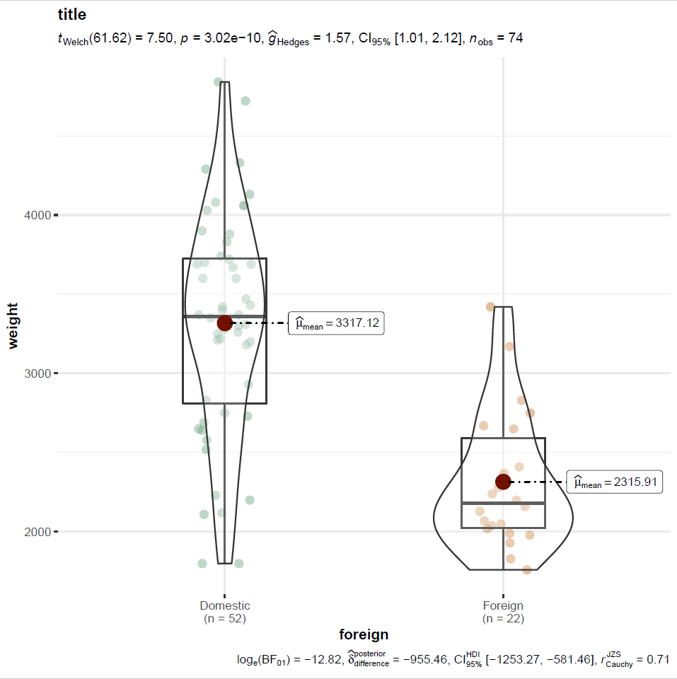
// let's make a violin plot using ggstatsplot
rcall: f <- ggbetweenstats( data = data, x=foreign, y=weight, title="title")
rcall: ggsave("ggstatsplottest.png", plot=f)
// figure out where that PNG is saved:
rcall: getwd()If you check your working directory (it was my “Documents” folder in Windows), you’ll find this figure as a PNG:
You can automate the output of ggstatsplot figures by editing the ggplot2 components that make it up. You’d insert the following into the ggstats plot code in the parentheses following “ggbetweenstats” to make the y scale on a log axis, for example:
ggplot.component = ggplot2::scale_y_continuous(trans='log') Quick do file to automate R-Stata integration and make ggplot2 or ggstatsplot figures
I made a do file that simplifies the setup of Rcall. Specifically, it 1. Sets R’s working directory to match your current Stata working directory, 2. Starts with a fresh R install, 3. Loads your current Stata dataset in R, and 3. Loads ggplot2 and ggstatsplot in R.
To use, just load your data, run a “do” command followed by the URL to my do file, then run whatever ggplot2 or ggstatsplots commands you want.This assumes you have installed R, the required packages, and Rcall (see very top of this page). If you get an error, try using this alternative version of the do file that doesn’t try to match Stata and R’s working directory.
Example code:
// Step 1: open dataset
sysuse auto, clear
// Step 2: run the do file, hosted on my UVM directory:
do https://www.uvm.edu/~tbplante/rcall_ggplot2_ggstatsplot_setup_v1_0.do
// if errors with above, use this do file instead:
// do https://www.uvm.edu/~tbplante/rcall_ggplot2_ggstatsplot_setup_alt_v1_0.do
// Step 3: run whatever ggplot2 or ggstatsplot code you want:
rcall: e<- ggplot(data, aes(x=mpg, y=weight)) + ///
	geom_point(aes(col=foreign, size=headroom)) + ///
	geom_smooth(method="loess") +   ///
	labs(title="ggplot2 demo", x="MPG", y="Weight", caption="Caption!")
rcall: ggsave("ggtest.png", plot=e)
Example 2: Using “comorbidity” R package in Stata with Rcall to estimate Charlson comorbidity index or Elixhauser comorbidity score
Read all about this handy package here and in the PDF reference manual. In R, type:
install.packages("comorbidity") Here’s some semicolon delimited Stata code to run from a Stata do file apply the Charlson comorbidity index to some Stata data.
webuse australia10, clear // load a default stata dataset with an ICD10 variable
gen id=_n // make an ID by row as there's no ID variable in this dataset

#delimit ;
rcall clear ;
rcall: library(comorbidity) ; // load comorbidity package
rcall: data<- st.data() ; // move data to r
rcall: names(data) ; // look at data
rcall: head(data, n=10) ; // look at rows
rcall: charlston <- comorbidity(x=data, id="id", code = "cause",
		map = "charlson_icd10_quan", assign0 = FALSE) ;
rcall: score(x=charlston, weights = "charlson", assign0=FALSE) ;
rcall: mergeddata <- merge(data, charlston, by="id") ; // merge the original & new charlson data
rcall: head(mergeddata, n=10) ; // look at rows
rcall: st.load(mergeddata) ; // kick the merged data back to stata
#delimit cr
Example 3: Predicting race by last name and sex by first name using the ‘predictrace’ package
I came across this ‘predictrace’ package: https://jacobkap.github.io/predictrace/
…which says that it implements the methods described in this paper:
- Tzioumis, K. Demographic aspects of first names. Sci Data 5, 180025 (2018). https://doi.org/10.1038/sdata.2018.25
- https://www.nature.com/articles/sdata201825
Here’s how to use this package in Stata using Rcall. There is a lot of nuance in this package so make sure to read the paper and the github page.
In R, type:
install.packages(predictrace)Then in Stata, write a do file that generates a variable called “lastnames” that is lower case last names (for race matching) and “firstnames” that is lowercase first names (for sex matching). Below is the code to estimate race by last name (first batch of code) and then sex by first name (second batch of code). This is semicolon delimited.
Estimating race by last name
(Note: this considers “Hispanic” to be a race and not an ethnicity…)
// Clear memory, input dataset of first and last names.
// Here, I'm formatting the strings so they are up to 100 characters
// in length so they don't get clipped (str100).
// If I specified str5 then "Flintstone" would be "Flint".
clear all
input str100 firstname str100 lastname
"Jacob" "Peralta"
"Rosa" "Diaz"
"Terrence" "Jeffords"
"Amy" "Santiago"
"Charles" "Boyle"
"Regina" "Linetti"
"Raymond" "Holt"
"Michael" "Hitchcock"
"Norman" "Scully"
end

compress firstname // optional, shortens string format from 100 char to the minimum length
compress lastname // optional, shortens string format from 100 char to the minimum length

// now replace all names with their lower case variant:
replace firstname = lower(firstname) // first name isn't used here fyi
replace lastname = lower(lastname)

#delimit ;
rcall clear ;
rcall: library(predictrace) ; // load predictrace
rcall: data<- st.data() ; // move data to r
rcall: names(data) ; // look at names of data
rcall: head(data, n=10) ; // look at first 10 rows
rcall: lastnamevector <-data[, "lastname"] ; // make vector from lastname column
rcall: data = merge(data, predict_race(lastnamevector), by.x = 'lastname', by.y = 'name', sort = FALSE) ;
rcall: head(data, n=10) ; // look at rows
rcall: st.load(data) ; // kick the merged data back to stata
#delimit cr
Estimating sex by first name
// Clear memory, input dataset of first and last names.
// Here, I'm formatting the strings so they are up to 100 characters
// in length so they don't get clipped (str100).
// If I specified str5 then "Flintstone" would be "Flint".
clear all
input str100 firstname str100 lastname
"Jacob" "Peralta"
"Rosa" "Diaz"
"Terrence" "Jeffords"
"Amy" "Santiago"
"Charles" "Boyle"
"Regina" "Linetti"
"Raymond" "Holt"
"Michael" "Hitchcock"
"Norman" "Scully"
end

compress firstname // optional, shortens string format from 100 char to the minimum length
compress lastname // optional, shortens string format from 100 char to the minimum length

// now replace all names with their lower case variant:
replace firstname = lower(firstname)
replace lastname = lower(lastname) // last name isn't used here fyi

#delimit ;
rcall clear ;
rcall: library(predictrace) ; // load predictrace
rcall: data<- st.data() ; // move data to r
rcall: names(data) ; // look at names of data
rcall: head(data, n=10) ; // look at first 10 rows
rcall: firstnamevector <-data[, "firstname"] ; // make vector from firstname column
rcall: data = merge(data, predict_gender(firstnamevector), by.x = 'firstname', by.y = 'name', sort = FALSE) ;
rcall: head(data, n=10) ; // look at rows
rcall: st.load(data) ; // kick the merged data back to stata
#delimit cr
Special thanks to Katherine Wilkinson for her R brilliance in debugging this.
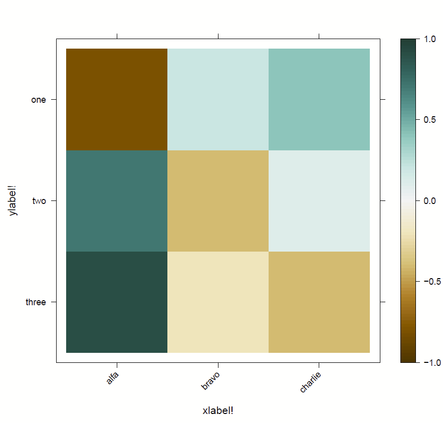
Example 4: Making a heatplot with lattice/levelplot
I wanted to make a heatplot ranging from -1 to +1 and wanted the negatives to be a different color from the positives, and have them turn more muted as they get to zero. I couldn’t quite figure out how to do this with the –twoway contour– or –plotmatrix– commands. It was pretty simple to do these in R, just needed to use the RColorBrewer package, specifying “BrBG” as the palette. I used the “lattice” package and its “levelplot” command as described in this post.
In R, install the lattice and RColorBrewer packages (lattice was already installed on my R desktop):
install.packages("lattice")
install.packages("RColorBrewer")
Now in Stata, input the data you’re interested in rendering in order of columns left to right then each column. Then, kick it to R, load the necessary libraries, grab your colorbrewer scheme of choice, label the axes, and then use the “levelplot” to render this. It will save a PDF in your R working directory. I couldn’t for the life of me figure out how to save it as a PNG but there was diminishing returns on figuring that out.
clear all
input x y z
-0.8 0.2 0.4
0.7 -0.4 0.1
0.9 -0.2 -0.4
end

#delimit ;
rcall clear ;
rcall: data<- st.data() ; // move data to r
rcall: names(data) ; // look at names of data
rcall: head(data, n=10) ; // look at first 10 rows
rcall: library(lattice) ; // load packages
rcall: library(RColorBrewer) ;
rcall: colors <- colorRampPalette(brewer.pal(16, "BrBG")) ; // get colors
rcall: colnames(data) <-c("alfa", "bravo", "charlie") ; //names of columns and rows
rcall: rownames(data) <-c("one", "two", "three") ;
rcall: levelplot(
		t(data[c(nrow(data):1) , ]),
		col.regions=colors,
		xlab="xlabel!",
		ylab="ylabel!",
		at=seq(min(-1), max(1), length.out=100),
		scales=list(y=list(rot=0), x=list(rot=45))
	) ; // pull data, apply colors & labels, set color axis range, rotate labels
rcall: getwd() ; // figure out where that PDF is saved:
#delimit cr
Here’s your output!