Getting the population, exposure, and outcome correct in your analytical dataset, and being able to come back and fix goofs later

Defining a study population, exposure variable, and outcome variable is a critical early step after determining your analysis plan. Most epidemiology projects come as a huge set of datasets, and you’ll probably need to join multiple files into one when defining your analytical population. Defining your analytical population is an easy place to make errors so you’ll want to have a specific script that you can come back and edit again if and when you find goofs.

For the love of Pete — Please generate your population, exposure, and outcome variables using a script so you can go back and reproduce these variables and fix any bugs you might find!

When you make these variables, you’ll likely need to combine several datasets. This will require mastery of importing datasets (if not in the native format for your statistical program) and combining datasets. For Stata, this means using –import– and –save– commands to bring everything over into Stata format, and then using –merge– commands to combine multiple datasets.

Make a variable for your population that is 0 (not included) or 1 (included)

One option in generating your dataset is to drop everyone who isn’t in your dataset. I recommend against dropping individuals who aren’t in your dataset. Instead, create a variable to define your population. Name it something simple like “included”, “primary population”, “group_a” or whatnot. If you will have multiple populations (say, one defined by prevalent hypertension using JNC7 vs. ACC/AHA 2017 hypertension thresholds), then you should have a variable for each addended with a simple way to tell them apart. Like “group_jnc7” and “group_aha2017”.

Useful code in R and Stata to do this:

• Count
• Generate and replace (Stata), mutate (R)
• Combine these with assigning single equals sign “=” (Stata & R, I say out loud “assign” when using this) and “<-" (R)
• use –if–, –and–, & –or– statements
• Tests of equality: >, =, <=, != (not), == ("equals exactly"), not single equal sign

Example Stata code to count # of people with diabetes, generate a variable for group_a and assign someone to group_a if they have diabetes.

count if diabetes==1
gen group_a=0
replace group_a=1 if diabetes==1

Here’s example R code to do the same (df=data frame).

nrow( df %>% filter(diabetes == 1) )
df = df %>% mutate(group_a = ifelse(diabetes == 1, 1, 0) )

Make an inclusion flowchart

These are essential charts in observational epidemiology. As you define your population, generate this sort of figure. Offshoots of the nodes define why folks are dropped from the subsequent node. Here’s how I approach this, folks might have different approaches:

• Node 1 is the overall population.
• Node 2 is individuals who you would not drop for baseline eligibility reasons (had prior event that discounts them or missing data to prevent assessment of their eligibility)
• Node 3 is individuals who you would not drop because you can assess them for necessary follow-up (incomplete follow-up, died before required follow-up time, missing data)
• Node 4 is individuals who you would not drop because they had all required exposure covariates (if looking at stroke by cholesterol level, people who all have cholesterol). This is your analytical population.

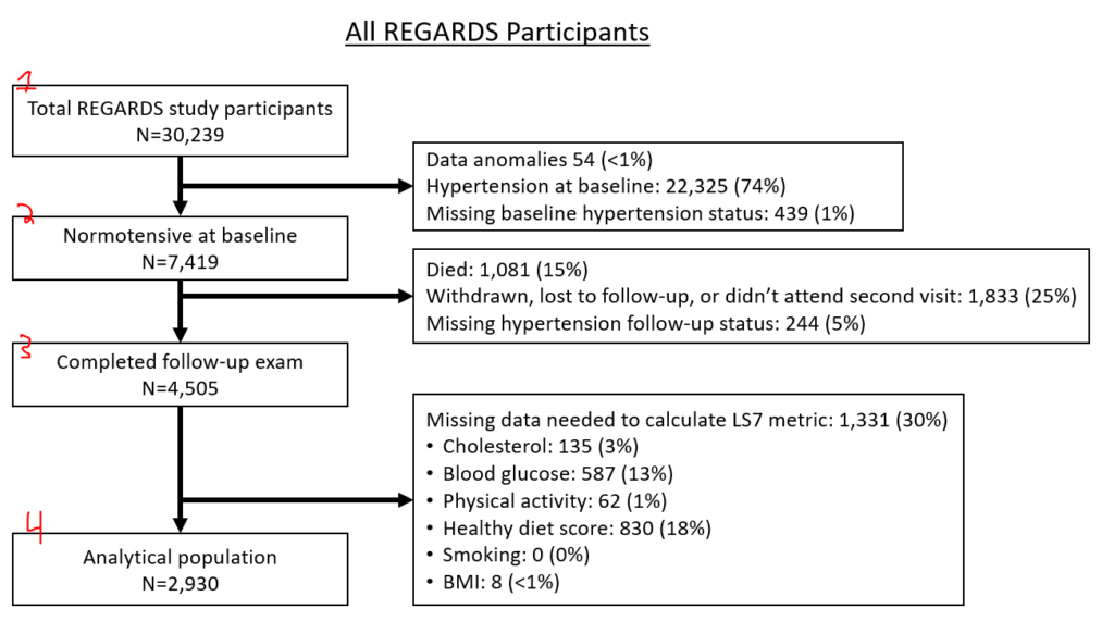
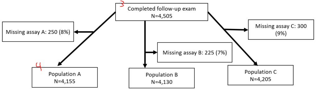
If you have two separate populations (eg, different hypertension populations by JNC7 or ACC/AHA 2017), you might opt to make two entirely separate figures. If you have slightly different populations because of multiple exposures (e.g., 3 different inflammatory biomarkers, but you have different missingness between the 3), you might have the last node fork off into different nodes, like this:

I generate these via text output in Stata then manually generate them in PowerPoint.

Defining exposure and outcome

This seems simple, but define clearly what your exposure is and your outcome is. Each should have a simple 0 or 1 variable (if dichotomous) with an intuitive name. You might need 2 separate outcomes if you are using different definitions, like “incident_htn_jnc7” and “incident_htn_aha2017”.

Table 1

“Table 1” shows core features of the population by the exposure. Don’t include the outcome as a row, but include demographics and key risk factors/covariates for outcome (eg if CVD, then diabetes, blood pressure, cholesterol, etc.). Some folks include a 2nd column that presents the N for that row. Some folks also include a P-value comparison as a final row. I tend to generate the P value every time but only present it if the reviewers ask for it.

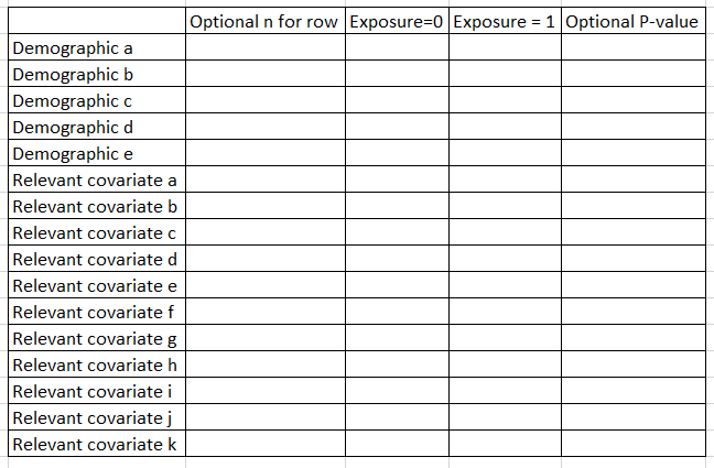
In Stata, I use the excellent table1_mc program to generate these, which you can read about here. For R, I am told that gtsummary works well.