What’s in a Table 1?
Baseline demographic tables (colloquially known as ‘Table 1’ given their common location) are a core feature of nearly all epidemiologic manuscripts. The columns represent the exposure you are studying. The rows are characteristics of your population that are relevant to your research project. In placebo-controlled RCTs, the columns are drug and placebo. In observational studies, the column is your exposure of interest. Say you are curious about the relationship between smoking and development of breast cancer in a cohort. Here, the columns would be smoking and no smoking.
Wait, I’m looking at a Table 1 has more than just a column for each exposure!
There are certain variations that you’ll see in Table 1s:
- A row for the entire population – This always seems overkill to me.
- A row with P-values – These are of no value in RCTs in my opinion. They are only occasionally helpful in observational studies.
The ultimate design of the Table 1 will be dictated by the target journal. This creates challenges for authors, who may need to rework Table 1s in the submission (and resubmission) process.
Why have Table 1s historically been such a pain in the butt to make in Stata?
Well, Stata doesn’t natively pop out Table 1s. Formulating one either requires manually running –sum– commands over and over again or writing custom code to help automate this for you.
Enter table1_mc
The Stata program table1_mc was released by Mark Chatfield, a biostatistician at the University of Queensland. It’s a derivation of the original table1 program by Phil Clayton. It’s a work of wonder. It automates the generation of a Table 1 with a few simple codes. Need to reformat for a new target journal? Make minor changes and hit re-run and — ”POOF”’ — out pops an updated and compliant Table 1.
Step 1: Install the program
Type:
ssc install table1_mcStep 2: Label your variables
Pluck out the variables you’ll include as the exposure and outcome. The table1_mc code will apply your bizarre, space-less variable name to the output unless you are using labels. Use real capitalization and formatting like you’d want to appear.
Step 2a: Labeling the variable itself
Let’s say you want to label your systolic blood pressure variable ‘sbp’ to be ‘Systolic blood pressure, mm Hg’. Type:
label variable sbp "Systolic blood pressure, mm Hg" Step 2b: Labeling the categories within variables
My suggestion is to generate a numerical ordinal variable and apply the labels to a number. The table1_mc program will put things in alphabetical or numerical order. Applying labels to numbers makes it easy to control the order. In this example, I have labels for income that I’ll make into a numerical ordinal variable first. In the raw dataset, the variables are defined using strings like “$20k-$34k”.
gen income1234=.
replace income1234=1 if income_4cat=="less than $20k"
replace income1234=2 if income_4cat=="$20k-$34k"
replace income1234=3 if income_4cat=="$35k-$74k"
replace income1234=4 if income_4cat=="$75k and above"
replace income1234=99 if income_4cat=="Refused"
Now,
1. Define the labels that you want to apply to income1234’s values of 1, 2, 3, 4, or 99, and
2. Apply the stupid labels. I always forget to apply the labels to the categorical values.
label define income_labels 1 "<$20K" 2 "$20k-$34k" 3 "$35k-$74k" 4 "$75k and above" 99 "Refused" // define the labels
label values income1234 income_labels // apply the labels!!
And, while you’re at it, don’t forget to apply a label to the overall ‘income1234’ variable that you made.
label variable income1234 "Annual household income"Step 3: Make a table 1
The help document (type ‘help table1_mc’) is a must read. Please look at it.
First: Start with ‘table1_mc,’ then the exposure expressed as ‘by(EXPOSURE VARIABLE NAME)’. Then just list out the variables you want in each row one by one. Each variable should have an indicator for the specific data types:
- Binary:
- bin – binary with P-value from Pearson’s chi2
- bine – binary with P-value from Fisher’s exact
- Continuous:
- contn – normally distributed, continuous variable, which will give mean and SD
- contln – log-normally distributed, continuous variable, which will give geometric mean and GSD
- conts – other continuous variable, which will give median and IQR.
- Categorical:
- cat – categorical with P-value from Pearson’s chi2
- cate – categorical with P-value from Fisher’s exact
After the code telling Stata which format you are using, you tell it what output format you want it to report the variables. Stata defaults to a lot of decimals. If you don’t specify, mean age may be presented as ‘42.818742022’. What a mess.
You can probably do 99% of your formatting with two codes:
- %4.0f – four leading digits, nothing after the decimal (e.g., 43)
- %4.1f – four leading digits, one digits after the decimal (e.g., 42.8)
Next, separate each variable with a backslash (‘\’). I like to break each line using the three forward slashes after (‘///’) so that I don’t have one ungodly line of text.
FINALLY, tell it some key options at the end:
- Ones I recommend including every time:
- onecol – categorical variables will have a header that’s an extra leading row before they are presented, rather than a whole separate column.
- missing – this keeps missing variables included. Helpful to show missingness of categorical variables.
- nospace – this will drop dead spaces before single digit numbers. E.g., it’ll present ‘(3%)’ instead of ‘( 3%)’.
- saving – output the Table 1 to Excel. Make sure that the Excel file output is not open in an Excel window when trying to overwrite a table. Otherwise, Stata will not run and you will be sad.
- Simple things to help reformatting for journals:
- [nothing] – presents n (%)
- percent – presents a % alone without including the n
- percent_n – % (n)
- slashN – n/N instead of just n
- total(before) – leading row with overall baseline demographics.
Some actual code to run table1_mc!
* Below will check if table1_mc is installed, and if it isn't then
* it'll install it. These 2 lines are optional and can be deleted.
capture which table1_mc
if _rc==111 ssc install table1_mc
* now specify things by "myexposure"
table1_mc ///
if include==1 /// <--can delete if not needed
, ///
by(myexposure) ///
vars( ///
age contn %4.0f \ ///
sex0m1f bin %4.0f \ ///
race0w1b bin %4.0f \ ///
region123 cat %4.0f \ ///
educ1234 cat %4.0f \ ///
income1234 cat %4.0f \ ///
sbp contn %4.0f \ ///
dbp contn %4.0f \ ///
smoke7_ideal bin %4.0f \ ///
pa7_ideal bin %4.0f \ ///
diet7_ideal bin %4.0f \ ///
chol7_ideal bin %4.0f \ ///
fpg7_ideal bin %4.0f \ ///
bmi7_ideal bin %4.0f \ ///
bp7_ideal bin %4.0f \ ///
) ///
nospace percent onecol missing total(before) ///
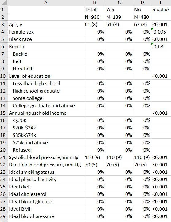
saving("table 1.xlsx", replace)…And here’s the (fake) result!
I’m working on an actual analysis right now so replaced all of the data from the actual output above with fake numbers. But you get the idea!