
What’s up with adding text to figures in Stata?
It’s handy to add text to your plots to orient your readers to specific observations in your figures. You might opt to highlight a datapoint, add percentages to bars, or say what part of a figure range is good vs. bad.
Adding text to Stata is relatively straightforward, once you get over the initial learning hump. Check out the added text help files by typing —help added_text_options— and —help textbox_options— for details.
Added text syntax
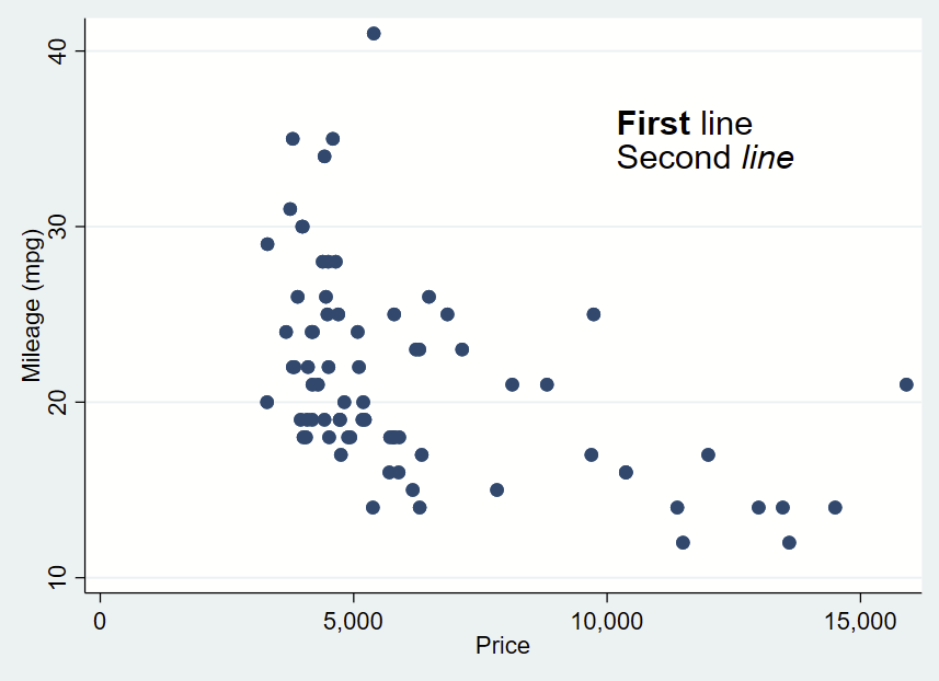
First, make your figure, then add your comma, then add your syntax. Like everything(?) in Stata, the location is specified as Y then X. Then add your text in quotes (or multiple quotes in a row if you want to insert a line break). You can bold or italicize by using the it: and bf: formatting and wrapping the text you want to apply it to in brackets. Then you drop a comma, specify placement as centered (c) or cardinal directions (e.g., ne, s, w) of that text box relative to the Y,X coordinates, justification of the text as left-aligned (left), centered (center), or right-aligned (right), and size of the text (vsmall, small, medsmall, medium, medlarge, large, vlarge, huge as shown in —help textsizestyle–).
Text box without outline, playing around with bolding and italicizing:
sysuse auto, clear
twoway ///
(scatter mpg price) ///
, ///
text(35 12000 "{bf:First} line" "Second {it:line}", placement(c) justification(left) size(large))
Text box with outline
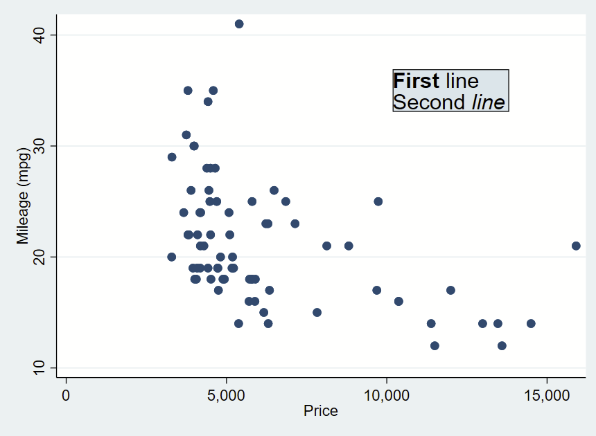
The main difference is that you add the word “box” to your text box options.
sysuse auto, clear
twoway ///
(scatter mpg price) ///
, ///
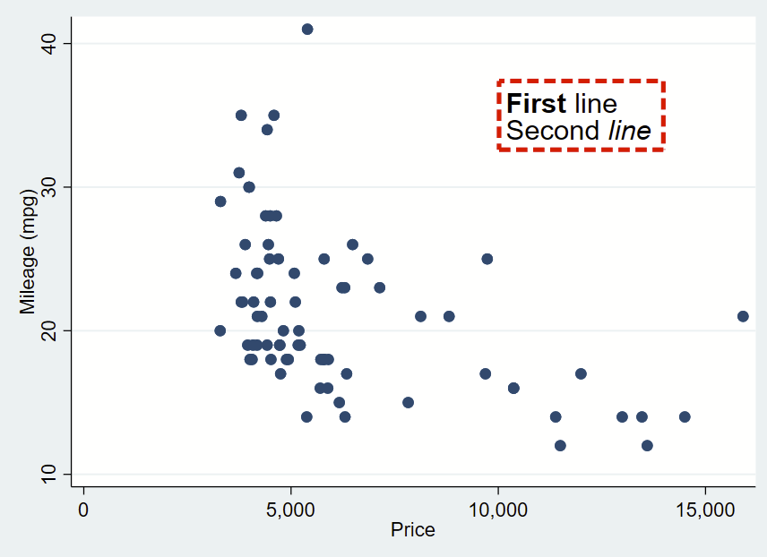
text(35 12000 "{bf:First} line" "Second {it:line}", placement(c) justification(left) size(large) box)You can further customize your box by specifying options shown under —help textbox_options–. Here, I’m making a box with no fill, and a thick/dashed/red outline with fcolor (fill color, which can be “none” for blank/see-through), lcolor (outline color), lpattern (outline pattern), and lwidth (thickness of outline).

sysuse auto, clear
twoway ///
(scatter mpg price) ///
, ///
text(35 12000 "{bf:First} line" "Second {it:line}", placement(c) justification(left) size(large) box fcolor(none) lcolor(red) lpattern(dash) lwidth(thick))
That looks pretty cool, but I’d like there to be more space between the text and the border. That’s specified with “margin”. There’s lots of complex options for this command you can read about in —help marginstyle–, but specifying “small” margin will add just a little buffer.
sysuse auto, clear
twoway ///
(scatter mpg price) ///
, ///
text(35 12000 "{bf:First} line" "Second {it:line}", placement(c) justification(left) size(large) box fcolor(none) lcolor(red) lpattern(dash) lwidth(thick) margin(small))
Special characters, and offsetting the Y,X coordinates
Sometimes you need a superscript 2 or 3, an arrow, or some other special character. Here are some that you can copy/paste into your text:
≥
≤
±
↑
↓
←
→
↔
🗸
χ² (chi-squared)
°
α
β
δ
Δ
γ
² (squared)
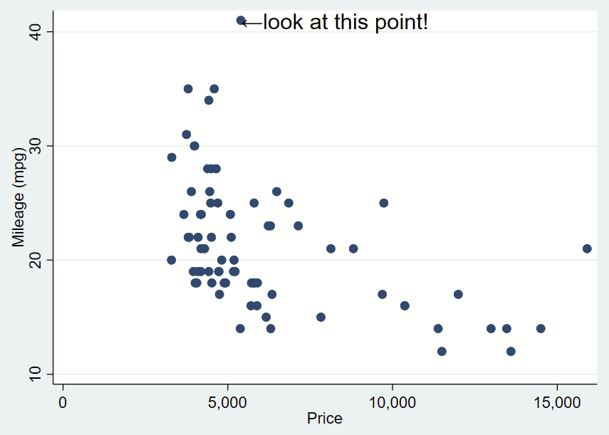
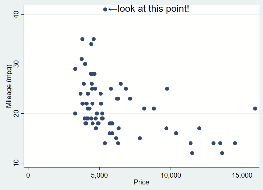
³ (cubed)Here’s how you might use the above arrow. Here, I’ve changed the placement to “e” for “east” so the text is to the right and centered of the specified Y,X coordinates of this point (which I looked up, it’s 41,5397). I’ve dropped the box and it’s only one line. I need to manually specify the Y,X coordinates, so it’s a bit clunky still.
sysuse auto, clear
twoway ///
(scatter mpg price) ///
, ///
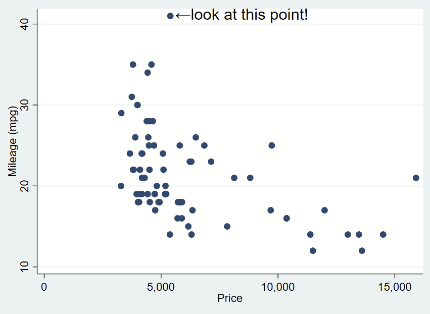
text(41 5397 "←look at this point!", placement(e) justification(left) size(large))You’ll notice that the left pointing arrow is inside the point of interest. The left pointing arrow in Ariel text isn’t exactly vertically centered (that’s a quirk of Ariel). You can “nudge” the text box to the right and up by adding an offset to the Y and X coordinates. To do math on an x,y point and add an offset, you place the point in an opening tick (to the left of 1 on your keyboard) and an apostrophe, and putting an equal sign at the beginning. After a bit of trial and error, we want to add an offset of +0.3 to the Y coordinate and +200 to the X coordinate.
sysuse auto, clear
twoway ///
(scatter mpg price) ///
, ///
text(`=41+0.3' `=5397+200' "←look at this point!", placement(e) justification(left) size(large))
If we want to automate the extreme numbers on either axis, we can use the sum command to grab the maximum value aka r(max) of the Y axis and the corresponding x value for that extreme. We can make a local macro to grab that value. Since this uses local macros, you need to run all lines at once in a do file, not line by line.
sysuse auto, clear
// grab yaxis (mpg) extreme
sum mpg, d
// now look at the r-value scalars we can call.
// note that r(max) is 41 and is the maximum.
return list
// now save r(max) as a local macro
local ymax = r(max)
// now let's find the x value for that y value.
// remember that the x axis variable is "price"
sum price if mpg==`ymax', d
// now look at r-value scalars you can call.
// since there's only 1 value, the mean, min, max,
// and sum are all the same.
return list
// let's now grab the r(mean) of as a local macro
local ymax_x = r(mean)
// now you can prove that you grabbed the correct point
di "Y max =" `ymax' ", and that point is at X=" `ymax_x'
// now place those local macros in the Y and X, keeping
// the other offsets
twoway ///
(scatter mpg price) ///
, ///
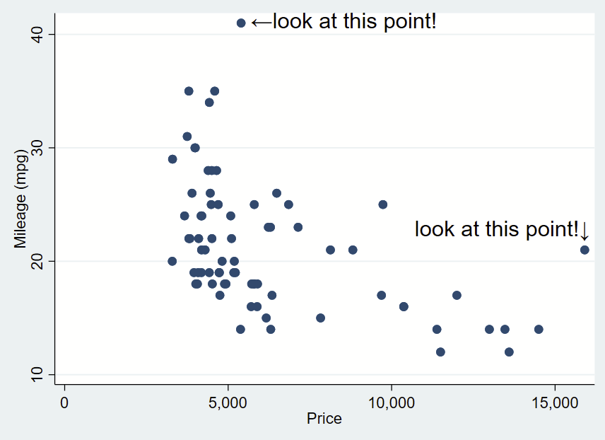
text(`=`ymax'+0.3' `=`ymax_x'+200' "←look at this point!", placement(e) justification(center) size(large))You can do the same for the x-axis extreme in the same script. for the X extreme, we’ll change the placement so it’s northwest and also tweak the Y,X coordinate offsets.
sysuse auto, clear
sum mpg, d
local ymax = r(max)
sum price if mpg==`ymax', d
local ymax_x = r(mean)
di "Y max =" `ymax' ", and that point is at X=" `ymax_x'
//
sum price, d
local xmax=r(max)
sum mpg if price==`xmax', d
local xmax_y=r(mean)
di "X max =" `xmax' ", and that point is at Y=" `xmax_y'

twoway ///
(scatter mpg price) ///
, ///
text(`=`ymax'+0.3' `=`ymax_x'+200' "←look at this point!", placement(e) justification(center) size(large)) ///
text(`=`xmax_y'+1' `=`xmax'+260' "look at this point!↓", placement(nw) justification(center) size(large))
What about adding text labels bar graphs?
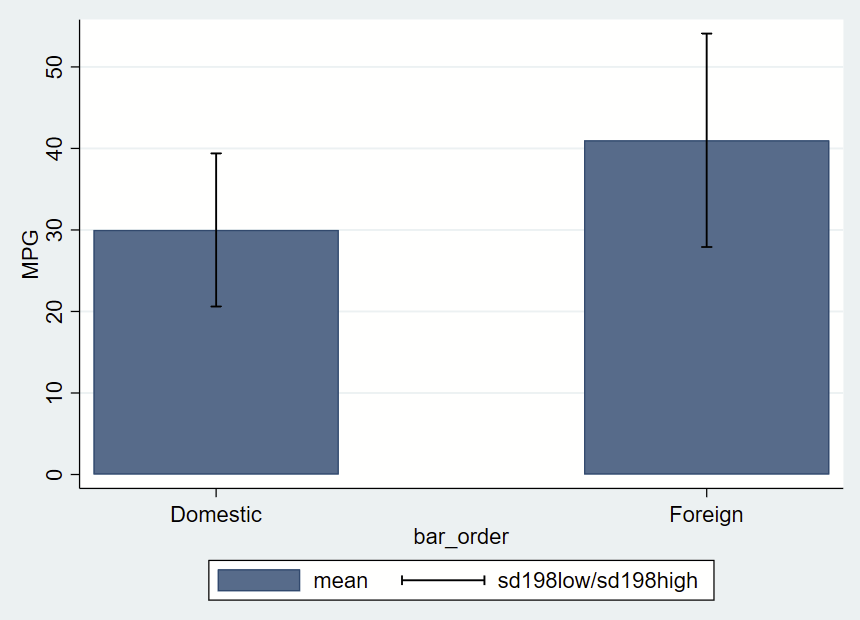
There’s a simple –graph bar– command, which isn’t terribly customizable. Here, we’ll be using the –twoway bar– bar graphs and add some fancy error bars with –twoway rcap–. The simplest way to do this is to make a new “dataset” from summary statistics in a separate frame. Frames are new in Stata 16, so if you are using an older version, this won’t work.
After making a frame with a bunch of summary statistics by group (most of which we won’t use here, but you might opt to later so we’ll keep it all there), you get this figure of mean and +/- 1.98*SD error bars.
// this has local macros so need to run from top to bottom in a do file!
// clear all frames
version 16
frames reset
sysuse auto, clear
// make a new frame called "bardata" that will store the values for bars.
frame create bardata str20 rowname n low95 high95 mean sd median iqrlow iqrhigh bar_order
//
// now grab summary statistics for foreign==0
// grab 2.5th and 95th %ile and save as local macros
// in case you might want them ever
_pctile mpg if foreign==0, percentiles(2.5 97.5)
local low95 = r(r1)
local high95= r(r2)
// now sum with detail one row
sum mpg if foreign==0, d
// post these to the new frame/bardata
// note the final row, which will be the x axis value that will correspond with bar placement
frame post bardata ("Foreign==0") (r(N)) (r(mean)) (`low95') (`high95') (r(sd)) (r(p50)) (r(p25)) (r(p75)) (1)
//
// now repeat for foreign==1
_pctile mpg if foreign==1, percentiles(2.5 97.5)
local low95 = r(r1)
local high95= r(r2)
sum mpg if foreign==1, d
// note the final row is now 3, leaving a gap of between the prior row
frame post bardata ("Foreign==1") (r(N)) (r(mean)) (`low95') (`high95') (r(sd)) (r(p50)) (r(p25)) (r(p75)) (3)
// now change to the frame with the summary statistics
cwf bardata
// let's make a new variable that's the mean +/- 1.98*sd
gen sd198low = mean-(sd*1.98)
gen sd198high = mean+(sd*1.98)
// now graph those data
twoway ///
(bar mean bar_order) ///
(rcap sd198low sd198high bar_order, vert lcolor(black)) ///
, ///
yla(0(10)50) ///
xla(1 "Domestic" 3 "Foreign") ///
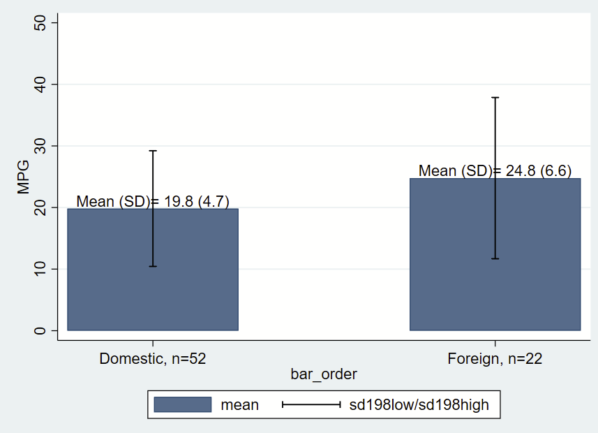
ytitle("MPG") Let’s make things a bit more fancy with labels, and place a text box with the mean and SD immediately above/north of the bars, which themselves are means of MPG by group. One quirk of Stata is that when formatting printed text from stored values, you need to place the label in an opening and closing tick, put a colon, type display, then apply the formatting (e.g., %3.1f for 1 digit after the decimal) then the value you are trying to show. You’ll notice that formatting in the last two lines of the following code.
// clear all frames
version 16
frames reset
sysuse auto, clear
// make a new frame called "bardata" that will store the values for bars.
frame create bardata str20 rowname n mean low95 high95  sd median iqrlow iqrhigh bar_order
//
// now grab summary statisticis for foreign==0
// grab 2.5th and 95th %ile and save as local macros
_pctile mpg if foreign==0, percentiles(2.5 97.5)
local low95 = r(r1)
local high95= r(r2)
// now sum with detail one row
sum mpg if foreign==0, d
// post these to the new frame/bardata
// note the final row, which will be the x axis value that will correspond with bar placement
frame post bardata  ("Foreign==0") (r(N)) (r(mean)) (`low95') (`high95') (r(sd)) (r(p50)) (r(p25)) (r(p75)) (1)
//
// now repeat for foreign==1
_pctile mpg if foreign==1, percentiles(2.5 97.5)
local low95 = r(r1)
local high95= r(r2)
sum mpg if foreign==1, d
// note the final row is now 3, leaving a gap of between the prior row
frame post bardata  ("Foreign==1") (r(N)) (r(mean)) (`low95') (`high95') (r(sd)) (r(p50)) (r(p25)) (r(p75)) (3)

// now change to the frame with the summary statistics
cwf bardata
// let's make a new variable that's the mean +/- 1.98*sd
gen sd198low = mean-(sd*1.98)
gen sd198high = mean+(sd*1.98)

// let's grab the mean and SD for each group. This frame has only two
// rows of data, so we'll use the row notatition to generate a local from
// the first and second rows, with row number specified in brackets
local group0_mean = mean[1]
local group0_sd =sd[1]
local group0_n = n[1]
// print to check your work
di "for group 0, mean =" `group0_mean' ", SD=" `group0_sd' ", n=" `group0_n'
// do the other group
local group1_mean = mean[2]
local group1_sd =sd[2]
local group1_n = n[2]
// print to check your work
di "for group 1, mean =" `group1_mean' ", SD=" `group1_sd' ", n=" `group1_n'

// now graph those data
// we'll add labels for the mean and SD and also
// label the N in the xlabels
twoway ///
(bar mean bar_order) ///
(rcap sd198low sd198high bar_order, vert lcolor(black)) ///
, ///
yla(0(10)50) ///
xla(1 "Domestic, n=`group0_n'" 3 "Foreign, n=`group1_n'") ///
ytitle("MPG") ///
text(`group0_mean' 1 "Mean (SD)= `: display %3.1f `group0_mean'' (`: display %3.1f `group0_sd'')", placement(n)) ///
text(`group1_mean' 3 "Mean (SD)= `: display %3.1f `group1_mean'' (`: display %3.1f `group1_sd'')", placement(n))