New in MS Word 365 is Read Aloud. It’s a pretty straightforward, stripped down/simplified text-to-speech (TTS) tool. If you have dyslexia or otherwise are having a difficult time finding typos in your work, try this feature. It’s very helpful.

To turn it on, just head over to the Review tab and click on the Read Aloud button.

It’ll automatically start reading from your cursor forward. Traditional icons for audio playback will float in the top right corner of your document window. These include play/pause, skip back (one paragraph), ad skip forward (one paragraph).

There is an icon of a dude with radio waves coming out of his head. That’s the settings button.

I like cranking the speed up by a few notches. You can also switch to other installed voices. I’m a fan of David’s sonorous speech. I’d totally pay a few bucks to have a Gilbert Gottfried voice though.

What if you have an older version of MS Word? Well, before this feature was released, I was using WordTalk v4.3. It’s a free, standalone app from the folks at the University of Edinburgh. It has some nice keyboard shortcuts that you can enable. The interface is very klunky though. In a pinch, it’ll do the trick.

2017-09-28 update

After using Read Aloud consistently for the past month, I still enjoy and recommend its use. However, I find it to be a bit glitchy with documents that have many co-author comments or embedded references from Zotero. In these documents, the playback will stop mid-word on occasion.

There are also some keyboard shortcuts for Read Aloud, documented here:

• CTRL+Alt+Space – Start or quit Read Aloud
• CTRL+Space – Play/pause
• CTRL+Left arrow or CTRL+Right arrow – Skip back or forward a paragraph
• Alt+Left or Alt+Right – Decrease or increase reading speed

2017-11-08 update

I received a new computer that ships with MS Office 2016, not 365. Read Aloud isn’t in Office 2016. It turns out that you can enable the older Text-to-Speech functionality in a pinch. If you don’t have the MS Speech Platform installed, you can download it here.

First, right click on the ribbon and select “customize the ribbon”.

Next, make a new group under the Review tab. I called mine Speak. Then under Choose Commands From, select All Commands. Scroll down to Speak and add it to your new group called Speak. Hit save.

You should now have a Speak button on your Review tab. Highlight what you want it to read and click Speak. Click it again to stop the reading.

You can adjust the reading speed under the Windows Control Panel –> Speech Recognition –> Text to Speech (on the left).

I’m not an organized person by nature. However, I’m the kind of guy that likes to implement systems to overcome problems. In medical school, I didn’t have any sort of structure for my projects and found it frustrating to find the most recent versions of papers, posters, and other writings. Here’s an approach that I started using in fellowship that works for me.

Step 1: Save all of your work in one folder

This seems pretty obvious, but modern operating systems, cloud-based storage systems, and network drives all compete for your documents. If you are a windows user, I’m willing to bet that you have different projects saved on the Desktop, in your My Documents folder, in your cloud storage, and in your email in/outboxes. You probably also have alternate working drafts of your writings on different computers. This is a recipe for disaster.

Instead, make one folder that is accessible from your usual workstation. Call it Work, or something more creative. Save freaking everything in your Work folder from now until the end of time. 

Step 2: Make subfolders for different types of your work

Within your Work folder, make a subfolder for each flavor of project that you do. I have individual folders for Grants, Editorials, Non research (for blog posts and other miscellaneous work), and Research.

Step 3: Numerically and descriptively label each of your projects in its own sub-subfolder

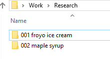
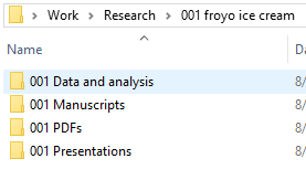
Let’s say you are about to have your first meeting for a new research project studying the effects of Fro-yo vs. ice cream on cholesterol among adults. All of the relevant documents for your next research project will now be saved in the 001 froyo ice cream folder, seen here:

(You also had a good idea for a maple syrup study that you have also started simultaneously.)

What is the threshold to start a new numerically and descriptively labeled sub-subfolder? Mine is pretty low. If I think I have at least a marginally good idea and have started emailing folks about it, I go ahead and start a new folder. A PDF copy of those initial emails are often the first things that I save in that new numerically and descriptively labeled sub-subfolder. (I loathe MS Outlook but have to use it. Its search is terrible. Saving copies of important emails saves me some headache.)

What kinds of things are you going to save into these folders? That’s up to you. I recommend saving your literature searches, copies of relevant important emails, research proposals, and so on. I like to make sub-sub-subfolders with headings like Data and analysis, Manuscripts, PDFs (for relevant literature saved from your library’s journal subscriptions), and Presentations. You should probably number these folders to match the overall sub-subfolder number as well.

Step 4: Name each item within your sub-sub-subfolders starting with the a) sub-subfolder name, b) a short descriptor of the thing you are writing, and c) ending with a revision and version number 

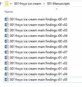
Example: You finished all of your awesome dessert-related research and are starting to write up the main findings. You are going to start your first MS Word version of the first draft. I suggest naming it like this: “001 froyo ice cream main findings r00 v01.docx“.

Using version numbers

The r00 (that’s r zero zero) means that this particular draft has never undergone a major revision from a prior draft. The v01 (that’s v zero one) means that it’s the first version ever. You’ll email out a file titled:

001 froyo ice cream main findings r00 v01.docx 

…to your primary collaborator who will send back something with edits, they’ll probably save it as:

001 froyo ice cream main findings r00 v01 BHO edits.docx

…which is nice but doesn’t help with your naming structure. Immediately save that to Work\Research\001 froyo ice cream\Manuscripts\ as version 02, or:

001 froyo ice cream main findings r00 v02.docx

Accept or refuse their edits and save that version as:

001 froyo ice cream main findings r00 v03.docx

…then send this out to more collaborators. You’ll wind up going through somewhere between 5-20 (or more) manuscript versions before you are ready to submit to a journal. What’s nice about this system is that you’ll have no problems figuring out which version of a file you are getting edits on. Remember, at >5 collaborators, the probability of one co-author checking their email <1 time per month approaches 100%. You'll be working on the 10th version of your draft and receive an email from the slow reviewer with edits to version 03. Sticking to this scheme helps you figure out how to integrate their suggestions into the current version by tracking the intermediate changes.

Note: I suggest using two digits (v01-v99) for the revision and version numbers rather than starting with 1 digit (v1-v99). This helps keeping files in alphabetical-numerical order when sorting in your file explorer. Computers aren’t smart enough to figure out that v12 doesn’t come between v1 and v2.

Using revision numbers

For some reason, the New England Journal of Medicine doesn’t accept your manuscript for publication after sending it out for review. Lucky for you, it was sent out for review and the reviewers gave you some high-quality feedback that will improve your paper. Now it’s time to start revision 01! When prepping it for the inevitable JAMA submission, you’ll be working starting on revision 01 and version 01, or:

001 froyo ice cream main findings r01 v01.docx 

In the end, you’ll have a folder looking like this:

Look at how pristine and well-organized this is!

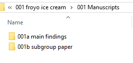
Step 4.5: Use trailing letters for projects with multiple publications

Let’s say that you decide to write both a main findings manuscript and a subgroup analysis manuscript. How to stay organized? Just the 001 Manuscripts folder into two sub-sub-sub subfolders for each publication, with 001a for the main findings and 001b for the subgroup analysis. It’ll look like this:

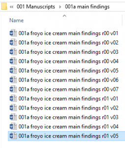
The naming scheme changes slightly as filenames will start with 001a instead of 001, like this:

Step 5: For the love of all things decent, regularly back up your Work folder!!

I can’t stress this enough. Keeping your Work folder in a commercial cloud storage drive doesn’t count as backing things up. Dropbox only saves things for 30 days in their basic plan. If you aren’t actively backing up your data, you can safely assume it isn’t backed up. One dead hard drive in a non-backed up folder can mean months or years of lost work.

Remember to check your institution’s policies for determining your backup method of choice. If you are working with PHI, saving it on an unencrypted thumb drive on your keychain won’t cut it. If it’s okay with your data policies, I recommend buying a DVD-R spindle or a bunch of cheap thumb drives and setting a calendar date to write your Work folder to a different DVD-R or different thumb drive once per month (i.e., you should have this on a different thumb drive each month). Keep these in a locked, secured, fireproof area that is consistent with the policies of your organization. Better yet, keep them in multiple locked, secured, fireproof areas if possible. For bonus points, get an M-Disc DVD discs and compatible burner, which should be stable for >1,000 years, unlike the usual 10-20 years of conventional burnable DVD-Rs and CD-Rs.

Or, just speak with your friendly neighborhood IT professional about how your institution recommends backing up the data you are working with. Chances are that they have a server that they back up 3 times per day that you can just use for a modest price. It’ll be worth the sorrow of lost data and drafts.

I’m a big fan of Tomighty. I have installed and used it extensively for the past year. It’s a simple timer for use with the Pomodoro technique. It helps maximize productivity and focus.

How I use the Pomodoro technique:

• Pick up a kitchen timer (like the ones crafted to resemble a tomato, or pomodoro in Italian).
• Get one sticky note and a pen. Stick the note to the right side of your desk. On the top, write “Pomodoros:”, a line down write “To do:”
• Close your email, put your phone on silent, and get away from all distractions.
• Set the timer for one Pomodoro (25 min).
• Work non-stop for that 25 minute span.
  • If a fleeting thought is vying to distract you during that timeframe (‘send this quick email‘, ‘remember to order some more pens‘, ‘double check that that meeting made it to my calendar‘, or ‘send that cute picture of my kid to grandma‘), jot it down on a sticky note for later.
• When your 25 min is up, count yourself one Pomodoro on the top of your sticky note.
• Set your timer for inter-Pomodoro time (5 min).
  • Do the simple tasks on your sticky note.
  • Say “BAM” every time you check one of those boxes on your to-do list.
    • Don’t worry about getting through them all in this 5 min span.
• When that 5 min is up, start your next Pomodoro.

The idea is to maximize the amount of Pomodoros you do in one day, not the duration of time that you work. Aim to get 3 your first day. Try to get up to 8 a week later. Only have an hour of time to work on one day? Do two Pomodoros.

With this technique, you stop counting minutes and hours and instead focus on bite-sized Pomodoros. As the day goes on and you rack up Pomodoros, you have fewer distracting thoughts and more productive time. For me, watching the clock causes a mild, counterproductive agitation. I don’t have this response counting Pomodoros.

This system helps you optimize your 1. Productivity requiring extended focus (writing papers, etc.), and 2. Productivity requiring little focus of silly things that you are putting off for later (quick emails, etc.).

In my opinion, the only drawback of the Pomodoro technique is the kitchen timer. It’s not quiet. Unless you have an office with a door and walls with soundproofing or work from home by yourself, this timer will cause problems with neighbors. Its not-so-quiet countdown/clicking and jarring ring will annoy folks in libraries, coffee shops, or cubicle communities.

Tomighty is a Java-based applet that replicates the tomato timer, written by Célio Cidral Junior. It has a lovely countdown click and time’s-up ring. It’ll keep track of your Pomodoros. It’s free and open source and should work on any computer (PC, Mac, Linux) with Java. Though, not the stock version of Java. I have struck out many times trying to figure out the correct version of Java to install and use. Every time I figure it out, I say “I should write this down.” Then I don’t. Fortunately, there is beta version written in C++ for Windows that doesn’t require Java. Just save the folder on your desktop and run the executable.