Part 8: Regressions

There are all sorts of models out there for performing regressions. This page focuses on 3 that are used for binary outcomes:

  1. Logistic regression
  2. Modified Poisson regression
  3. Cox proportional hazards models.

Getting set up

Before you get going, you want to explicitly define your outcome of interest (aka dependent variable), primary exposure (aka independent variable) and covariates that you are adjusting for in your model (aka other independent variables). You’ll also want to know your study design (eg case-control? cross-sectional? prospective? time to event?).

Are your independent variables continuous or factor/categorical?

In these regression models, you can specify that independent variables (primary exposure and covariates that are in your model) are continuous or factor/categorical. Continuous variables can be specified with a leading “c.”, and examples might include age, height, or length. (“c.age”.) In contrast, factor/categorical variables might be New England states (e.g., 1=Connecticut, 2=Maine, 3=Mass, 4=New Hampshire, 5=RI, and 6=Vermont). So, you’d want to specifiy a variable for “newengland” as i.newengland in your regression. Stata defaults to treating the smallest number (here, 1=Connecticut) as the reference group. You can change that by using the “ib#.” prefix instead, where the # is the reference group, or here ib2.newengland to have Maine as the reference group.

Read about factor variables in –help fvvarlist–.

What about binary/dichotomous variables (things that are ==0 or 1)? Well, it doesn’t change your analysis if you specify a binary/dichotomous as either continuous (“c.”) or factor/categorical (“i.”). The math is the same on the back end.

Checking for interactions

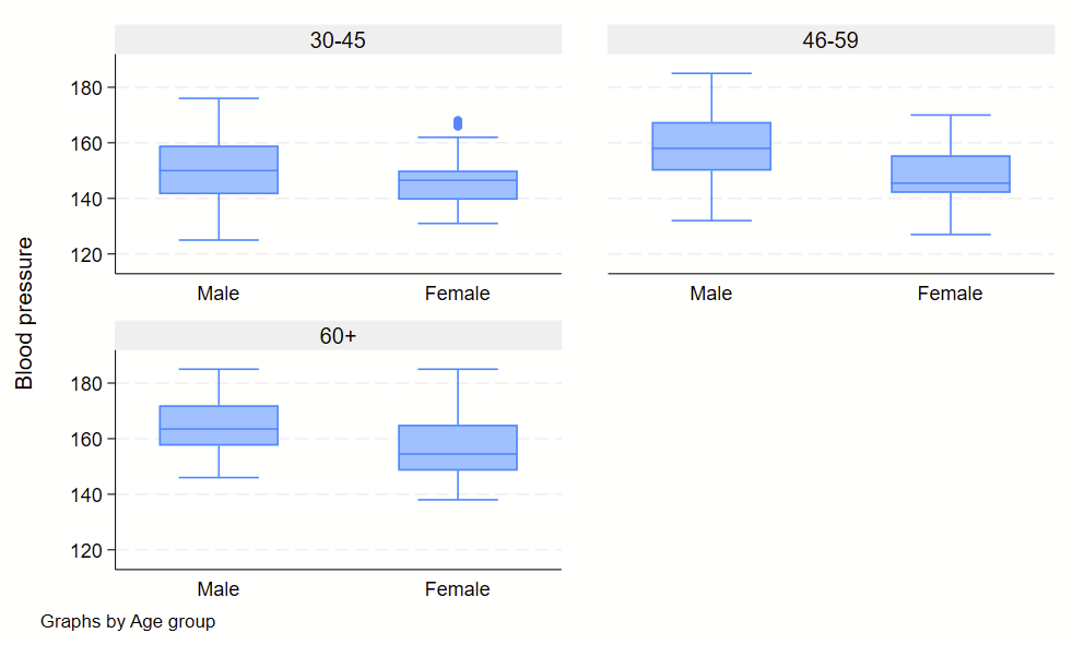
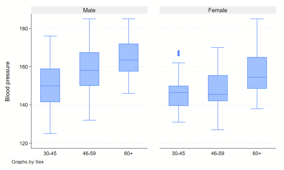
In general, when checking for an interaction, you will need to specify if the two variables of interest are categorical or factor/categorical and drop two pound signs in between the two. See details on –help fvvarlist–. Here’s an example of how this would look, looking for an interaction between sex on age groups.

regress bp i.sex##c.agegrp

      Source |       SS           df       MS      Number of obs   =       240
-------------+----------------------------------   F(3, 236)       =     23.86
       Model |   9519.9625         3  3173.32083   Prob > F        =    0.0000
    Residual |  31392.8333       236   133.02048   R-squared       =    0.2327
-------------+----------------------------------   Adj R-squared   =    0.2229
       Total |  40912.7958       239  171.183246   Root MSE        =    11.533

------------------------------------------------------------------------------
          bp | Coefficient  Std. err.      t    P>|t|     [95% conf. interval]
-------------+----------------------------------------------------------------
         sex |
     Female  |     -4.275   3.939423    -1.09   0.279    -12.03593    3.485927
      agegrp |     7.0625   1.289479     5.48   0.000      4.52214     9.60286
             |
sex#c.agegrp |
     Female  |      -1.35   1.823599    -0.74   0.460    -4.942611    2.242611
             |
       _cons |   143.2667   2.785593    51.43   0.000     137.7789    148.7545
------------------------------------------------------------------------------

You’ll see the sex#c.agegrp P-value is 0.460, so that wouldn’t qualify as a statistically significant interaction.

Regressions using survey data?

If you are using survey analyses (eg need to account for pweighting), generally you have to use the svy: prefixes for your analyses. This includes svy: logistic, poisson, etc. Type –help svy_estimation– to see what the options are.

Logistic regression

Logistic regressions provide odds ratios of binary outcomes. Odds ratios don’t approximate the risk ratio if the outcome is common (eg >10% occurrence) so I tend to avoid them as I study hypertension, which occurs commonly in a population.

There are oodles of details on logistic regression in the excellent UCLA website. In brief, you want want to use a regression command, you can use “logit” and get the raw betas or “logistic” and get the odds ratios. Most people will want to use “logistic” to get the odds ratios.

Here’s an example of logistic regression in Stata. In this dataset, “race” is Black/White/other, so you’ll need to specify this as a factor/categorical variable with the “i.” prefix, however “smoke” is binary so you can either specify it as a continuous or as a factor/categorical variable. If you don’t specify anything, then it is treated as continuous, which is fine.


webuse lbw, clear
codebook race // see race is 1=White, 2=Black, 3=other
codebook smoke // smoke is 0/1
logistic low i.race smoke 

// output: 
Logistic regression                                     Number of obs =    189
                                                        LR chi2(3)    =  14.70
                                                        Prob > chi2   = 0.0021
Log likelihood = -109.98736                             Pseudo R2     = 0.0626

------------------------------------------------------------------------------
         low | Odds ratio   Std. err.      z    P>|z|     [95% conf. interval]
-------------+----------------------------------------------------------------
        race |
      Black  |   2.956742   1.448759     2.21   0.027     1.131716    7.724838
      Other  |   3.030001   1.212927     2.77   0.006     1.382616     6.64024
             |
       smoke |   3.052631   1.127112     3.02   0.003     1.480432    6.294487
       _cons |   .1587319   .0560108    -5.22   0.000     .0794888    .3169732
------------------------------------------------------------------------------
Note: _cons estimates baseline odds.

So, here you see that the odds ratio (OR) for the outcome of “low” is 2.96 (95% CI 1.13, 7.72) for Black relative to White participants and the OR for the outcome of “low” is 3.03 (95% CI 1.38, 6.64) for Other race relative to White participants. Since it’s the reference group, you’ll notice that White race isn’t shown. But what if we want Black race as the reference? You’d use “ib2.race” instead of “i.race”. Example:

logistic low ib2.race smoke 
// output:

Logistic regression                                     Number of obs =    189
                                                        LR chi2(3)    =  14.70
                                                        Prob > chi2   = 0.0021
Log likelihood = -109.98736                             Pseudo R2     = 0.0626

------------------------------------------------------------------------------
         low | Odds ratio   Std. err.      z    P>|z|     [95% conf. interval]
-------------+----------------------------------------------------------------
        race |
      White  |   .3382101   .1657178    -2.21   0.027     .1294525    .8836136
      Other  |   1.024777   .5049663     0.05   0.960     .3901157    2.691938
             |
       smoke |   3.052631   1.127112     3.02   0.003     1.480432    6.294487
       _cons |   .4693292   .2059043    -1.72   0.085     .1986269    1.108963
------------------------------------------------------------------------------
Note: _cons estimates baseline odds.


Modified Poisson regression

Modified Poisson regression (sometimes called Poisson Regression with Robust Variance Estimation or Poisson Regression with Sandwich Variance Estimation) is pretty straightforward. Note: this is different from ‘conventional’ Poisson regression, which is used for counts and not dichotomous outcomes. You use the “poisson” command with subcommands “, vce(robust) irr” to use the modified Poisson regression type. Note: with svy data, robust VCE is the default so you just need to use the subcommand “, irr”.

As with the logistic regression section above, race is a 3-level nominal variable so we’ll use the “i.” or “ib#.” prefix to specify that it’s not to be treated as a continuous variable.

webuse lbw, clear
codebook race // see race is 1=White, 2=Black, 3=other
codebook smoke // smoke is 0/1
// set Black race as the reference group
poisson low ib2.race smoke, vce(robust) irr
// output:

Iteration 0:  Log pseudolikelihood = -122.83059  
Iteration 1:  Log pseudolikelihood = -122.83058  

Poisson regression                                      Number of obs =    189
                                                        Wald chi2(3)  =  19.47
                                                        Prob > chi2   = 0.0002
Log pseudolikelihood = -122.83058                       Pseudo R2     = 0.0380

------------------------------------------------------------------------------
             |               Robust
         low |        IRR   std. err.      z    P>|z|     [95% conf. interval]
-------------+----------------------------------------------------------------
        race |
      White  |    .507831    .141131    -2.44   0.015     .2945523    .8755401
      Other  |   1.038362   .2907804     0.13   0.893     .5997635      1.7977
             |
       smoke |   2.020686   .4300124     3.31   0.001     1.331554    3.066471
       _cons |   .3038099   .0800721    -4.52   0.000     .1812422    .5092656
------------------------------------------------------------------------------
Note: _cons estimates baseline incidence rate.

Here you see that the relative risk (RR) of “low” for White relative to Black participants is 0.51 (95% CI 0.29, 0.88), and the RR for other race relative to Black participants is 1.04 (95% CI 0.60, 1.80). As above, the “Black” group isn’t shown since it’s the reference group.

Cox proportional hazards model

Cox PH models are used for time to event data. This is a 2-part. First is to –stset– the data, thereby telling Stata that it’s time to event data. In the –stset– command, you specify the outcome/failure variable. Second is to use the –stcox– command to specify the primary exposure/covariates of interest (aka independent variables). There are lots of different steps to setting up the stset command, so make sure to check the –help stset– page. Ditto –help stcox–.

Here, you specify the days of follow-up as “days_hfhosp” and failure as “hfhosp”. Since follow-up is in days, you set the scale to 365.25 to have it instead considered as years.

stset days_hfhosp, f(hfhosp) scale(365.25)

Then you’ll want to use the stcox command to estimate the risk of hospitalization by beta blocker use by age, sex, and race with race relative to the group that is equal to 1.

stcox betablocker age sex ib1.race

You’ll want to make a Kaplan Meier figure at the same time, read about how to do that on this other post.

Part 7: Making a table for your outcome of interest (Table 2?)

As we learned in part 5, Table 1 describes your analytical population at baseline by your exposure. For those using a continuous variable as an exposure, it’s by quantile (e.g., tertile, quartile) of the exposure. I propose a table known as “Table 2” that describes the outcome of interest by the exposure used in Table 1. You might have seen something along the lines of this in papers before, and we are going to call it “Table 2”. It’s not a universal table in observational epidemiology, so calling it “Table 2” is a bit much. But we’ll call it “Table 2” for our purposes.

Columns

The columns should be identical to that in your Table 1. (I suggest having an “All” column if you don’t have one in your Table 1 though.)

Rows

In Table 1, I suggested having an N and range for continuous variables of your quantiles. I suggest not including those in your Table 2 if they are already in your Table 1, since it’s duplicative. I suppose it might be helpful for error checking to have them in table 2, and confirming that they are identical to your Table 1. But, I suggest not including a row for Ns and ranges in your Table 2 that is included in the manuscript.

In a very simple Table 2, there might be a single row: the outcome in the analytical population. It might look like this:

AllTertile 1Tertile 2Tertile 3
All

BUT! There might be a stratification of interest in your table. in the REGARDS study, we often stratify by Black vs. White race or by sex. So, you might also include rows for each subsequent group, like this:

AllTertile 1Tertile 2Tertile 3
All
Black participants
White participants

Finally, for subgroups, you might opt to include a minimally-adjusted regression comparing your strata. in this example, we could use a modified Poisson regression (i.e., Poisson regression with sandwich or robust variance estimators, Zou’s method) to compare risk of the outcome overall an in each tertile. I’d just adjust for age and sex in this example. So:

AllTertile 1Tertile 2Tertile 3
All
Black participants
White participants
RR, Black vs. White (ref)

Cell

Here, I suggest presenting # with event/# at risk (percentage with event) in each cell, except in the RR row, which would present RR and the 95% confidence interval. Example (totally made up numbers here and some placeholder ##’s, as FYI):

AllTertile 1Tertile 2Tertile 3
All1000/3000 (33%)300/1000 (30%)400/1000 (40%)500/1000 (50%)
Black participants400/1000 (40%)##/## (##%)##/## (##%)##/## (##%)
White participants600/2000 (30%)##/## (##%)##/## (##%)##/## (##%)
RR, Black vs. White (ref)1.25 (1.20-1.30)1.20 (1.15-1.25)1.22 (1.18-1.30)1.21 (1.19-1.28)

That’s it! Even if you don’t include this table, it’s super handy to have to describe the outcome in the text.

Part 6: Visualizing your continuous exposure at baseline

Visualization of your continuous exposure in an observational epidemiology research project

As we saw in Part 5, it’s important to describe the characteristics of your baseline population by your exposure. This helps readers get a better understanding of internal validity. For folks completing analyses with binary exposures, part 6 isn’t for you. If your analysis includes continuous exposures or ordinal exposures with at least a handful of options, read on.

I think it’s vitally important to visualize your exposure before moving any further forward with your analyses. There are a few reasons that I do this:

  1. Understand the distribution of your exposure. Looking at the raw spread of your data will help you understand if it has a relatively normal distribution, if it’s skewed, if it is multimodal (eg, has several peaks), or if it’s just plain old weird looking. If your exposure is non-normally distributed, then you’ll need to consider the implications of the spread in your analysis. This may mean log-transforming, square root-transforming (if you have lots of zeros in your exposure’s values), or some other sort of transformation.
    • Note: make sure to visualize your transformed exposure value!
  2. Look for patterns that need exploring. You might notice a huge peak at a value of “999”. This might represent missing values, which will need to be recoded. You might notice that values towards the end of the tails of the bell curve might spike up at a particular value. This might represent values that were really above or below the lower limit of detection. You’ll need to think about how to handle such values, possibly recoding them following the NHANES approach as the limit of detection divided by the square root of 2.
  3. Understand the distribution of your exposure by key subgroups. In REGARDS, our analyses commonly focus on racial differences in CVD events. Because of this, I commonly visualize exposures with overlaid histograms for Black and White participants, and see how these exposure variables differ by race. This could easily be done for other sociodemgraphics (notably, by sex), anthropometrics, and disease states.

Ways to depict your continuous exposure

  1. Stem and leaf plots
  2. Histograms
  3. Kernel density plots
  4. Boxplots

1. Stem and leaf plots

Stem and leaf plots are handy for quickly visualizing distributions since the output happens essentially instantaneously, whereas other figures (e.g., histograms) take a second or two to render. Stem and leaf plots are basically sideways histograms using numbers. The Stata command is –stem–.

* load the sysuse auto dataset and clear all data in memory
sysuse auto, clear
* now render a stem and leaf plot of weight
stem weight

Here’s what you get in Stata’s output window. You’ll see a 2 digit number (eg “17**”) followed by a vertical bar then another 2 digit number (eg “60”). That means that 1 person has a value of 1760. If there are multiple numbers after the bar, then that means that there are more than 1 number in that group. For example, the “22**” stem has “00”, “00”, “30”, “40”, and “80” leaves, meaning that there is 2200, 2200, 2230, and 2280 as values in this dataset.

Stem-and-leaf plot for weight (Weight (lbs.))

  17** | 60
  18** | 00,00,30
  19** | 30,80,90
  20** | 20,40,50,70
  21** | 10,20,30,60
  22** | 00,00,30,40,80
  23** | 70
  24** | 10
  25** | 20,80
  26** | 40,50,50,70,90
  27** | 30,50,50
  28** | 30,30
  29** | 30
  30** | 
  31** | 70,80
  32** | 00,10,20,50,60,80
  33** | 00,10,30,50,70,70
  34** | 00,20,20,30,70
  35** | 
  36** | 00,00,70,90,90
  37** | 00,20,40
  38** | 30,80
  39** | 00
  40** | 30,60,60,80
  41** | 30
  42** | 90
  43** | 30
  44** | 
  45** | 
  46** | 
  47** | 20
  48** | 40

For stems with a huge amount of values, you’ll see some other characters appear to split up the stem into multiple stems. For example, here’s the output for stem of MPG:

. stem mpg

Stem-and-leaf plot for mpg (Mileage (mpg))

  1t | 22
  1f | 44444455
  1s | 66667777
  1. | 88888888899999999
  2* | 00011111
  2t | 22222333
  2f | 444455555
  2s | 666
  2. | 8889
  3* | 001
  3t | 
  3f | 455
  3s | 
  3. | 
  4* | 1

You’ll notice that the 10-place stem is split into 4 different stems, “1t”, “1f”, “1s”, and “1.”. I’m guessing that *=0-1, t=2-3, f=4-5, s=6-7, .=8.9.

2. Histograms

A conventional histogram splits continuous data into several evenly-spaced discrete groups called “bins”, and visualizes these discrete groups as a bar graph. These are commonly used but in Stata can’t be used with pweighting. See kernel density plots below for consideration of how to use pweighting.

Let’s see how to do this in Stata, with some randomly generated data that approximates a normal distribution. While we’re at it, we’ll make a variable called “group” that’s 0 or 1 that we’ll use later. (Also note that this dataset doesn’t use discrete values, so I’m not specifying the discrete option in my “hist” code. If you see spaces in your histogram because you are using discrete values, add “, discrete” after your variable name in the histogram line.)

clear all
// set observations to be 1000:
set obs 1000
// set a random number seed for reproducibility: 
set seed 12345
// make a normally-distributed variable, with mean of 5 and SD of 10:
gen myvariable = rnormal(5,10)
// make a 0 or 1 variable for a group, following instructions for "generate ui":
// https://blog.stata.com/2012/07/18/using-statas-random-number-generators-part-1/
gen group = floor((1-0+1)*runiform() + 0)
// now make a histogram
hist myvariable

Here’s the overall histogram:

On the X axis you see the ranges of the values of variable of interest, from around -30 to about +40. On the Y axis you see the density plot. I want to show this same figure by group, however, and the bins are not currently transparent. You won’t be able to tell one group from another. So, in Stata, you need to use the “twoway histogram” option instead of just “histogram” and specify transparent colors of the figure using the %NUMBER notation. We’ll also add a legend. We’ll set the scheme to s1mono to get rid of the ugly default blue surrounding box as well. Example:

// set the scheme to s1mono:
set scheme s1mono
// now make your histogram:
twoway ///
(hist myvariable if group==0, color(blue%30)) ///
(hist myvariable if group==1, color(red%30)) ///
, ///
legend(order(1 "Group==0" 2 "Group==1"))

Here’s what you get:

You can modify things as needed. Something you might consider is changing the density to count or frequency, which is done by adding “frequency” or “percent” after the commas but before the colors. You might also opt to select different colors, which you can read about selection of colors in this editorial I wrote with Mary Cushman.

Considerations for designing histograms

One question is how many bins you want. I found this nice 2019 article by Regina L. Nuzzo, PhD (PDF link, PubMed listing) that goes over lots of considerations for the design of histograms. I specifically like the Box, which lists equations to determine number of bins and bid width. In general, if you have too many bins, your data will look choppy:

// using 100 bins here
twoway ///
(hist myvariable if group==0, color(blue%30) bin(100)) ///
(hist myvariable if group==1, color(red%30)  bin(100)) ///
, ///
legend(order(1 "Group==0" 2 "Group==1"))

And if you have too few, you won’t be able to make sense of the overall structure of the data.

// using 2 bins here
twoway ///
(hist myvariable if group==0, color(blue%30) bin(2)) ///
(hist myvariable if group==1, color(red%30)  bin(2)) ///
, ///
legend(order(1 "Group==0" 2 "Group==1"))

Be thoughtful about how thinly you want to splice your data.

What about histograms on a log scale?

You might have some sort of skewed variable that you want to show on a log scale. The easiest way to do this is to (1) make a log-transformed variable of this, and (2) make a histogram of the log-transformed variable. For part #2, you’ll want to print the labels of the original variable in their log-transformed spot, otherwise you’ll wind up with labels for the log-transformed variable, which are usually not easy to interpret. See the `=log(number)’ trick below for how to drop non-log transformed labels in log-transformed spots.

// clear dataset and make skewed variable
clear all 
set obs 1000
gen variable = 10+ ((rbeta(2, 10))*100)

// visualize non-log transformed data
twoway /// 
(hist variable) ///
, ///
xlab(10 "10" 20 "20" 30 "30" 40 "40" 50 "50" 60 "60")

// make a long-transformed variable
gen logvariable=log(variable)

// visualize non-log transformed data
// plop the labels in the spots where the "original" labels should be
twoway ///
(hist logvariable) ///
, ///
xlab(`=log(10)' "10" `=log(20)' "20" `=log(30)' "30" `=log(40)' "40" `=log(50)' "50" `=log(60)' "60")

Here’s the raw variable.

Here is the histogram of the log transformed variable. Notice that the 10-60 labels are printed in the correct spots with the `=log(NUMBER)’ code above.

3. Kernel density plots

Kernel density plots are similar to histograms, except it shows a smoothed line over your data’s distribution. Histograms are less likely to hide outliers since kernel density plots can smooth over outliers. The code for a kernel density plot in Stata is nearly identical to the “twoway hist” code above.

twoway ///
(kdensity myvariable if group==0, color(blue%30)) ///
(kdensity myvariable if group==1, color(red%30)) ///
, ///
legend(order(1 "Group==0" 2 "Group==1"))

Output:

You can even combine histograms and kernel density plots!

twoway ///
(hist myvariable if group==0, color(blue%30)) ///
(hist myvariable if group==1, color(red%30)) ///
(kdensity myvariable if group==0, color(blue%30)) ///
(kdensity myvariable if group==1, color(red%30)) ///
, ///
legend(order(1 "Group==0" 2 "Group==1"))

I’ve never done this myself for a manuscript, but just showing that it’s possible.

Using kdens to make kernel density plots that use pweights

You might need to make kernel density plots that use pweighting. There’s a –kdens– package that allows you to do that, which requires –moremata– to be installed. Here’s how you can make a pweighted kernel density plot with kdens.

 // only need to install once:
ssc install moremata
ssc install kdens
// load nhanes demo code
webuse nhanes2f, clear
// now svyset the data and use kdens to make a weighted plot
svyset psuid [pw=finalwgt], strata(stratid)
twoway kdens weight [pw=finalwgt]

And you’ll get this!

4. Boxplots

Boxplots are handy at showing distributions of multiple groups all at once. This is a nice overview of what all of the bits of the figure means. Briefly, there’s a box that is the median and IQR. There are some lines sticking out that are the upper and lower adjacent lines, which are the 75th percentile + (1.5*the width of the IQR range) and 25th percentile – (1.5*the width of the IQR range). Dots outside these ranges are the outliers.

Making boxplots is simple in stata using the –graph box– command. My one piece of advice is to be aware of the by() and over() commands since they can help you stitch together boxplots in interesting ways. Example code follows.

sysuse bplong, clear

graph box bp
graph box bp, over(sex) 
graph box bp, by(sex) 
graph box bp, by(agegrp) over(sex)  
graph box bp, by(sex) over(agegrp) 

No subcommands

Subcommand: , over(sex)

Subcommand: , by(sex)

Subcommand: , by(agegrp) over(sex)

Subcommand: , by(sex) over(agegrp)

How I use the Zotero reference manager for collaborative grants or manuscripts

Why Zotero?

Zotero is an excellent and free reference manager that is my go-to for writing grants and manuscripts. It has some very handy features, like word processor plugins, web browser plugins that will grab PDF versions of documents if available, and ability to share “group libraries” with collaborators. It has all of the standard features of reference managers, like auto-formatting of references to meet submission requirements, automatic renumbering of in-line references, etc.

There are some silly things about Zotero’s initial setup that are important to get out of the way. For example, you don’t necessarily need to have a Zotero account to use Zotero (or at least you didn’t when I used it the first time). Make sure that you read about how to get set up with Zotero under the “Zotero” heading on this page. After you do that, come back here and read on!

How to use Zotero for collaborative projects

Zotero works well with MS Word and Google Docs. Examples here are taken from MS Word, but are also applicable to Google Docs. The main difference between Google Docs and MS Word is that the web browser plugin is also the Google Docs plugin. MS Word has a plugin separate from the web browser plugin. Regardless, whenever you use a Zotero plugin (eg the MS Word, Google Docs, or browser extensions), you also need to have the Zotero desktop app open. You’ll get an error if you try to insert a reference into a document or snag a reference from PubMed/a journal website if the Zotero desktop app isn’t also open.

Organizing your folders (“collections”) and subfolders (“subcollections”).

In your desktop app, navigate to the shared library that I’ll send you. Make folders/collections or subfolders/subcollections in there to help stay organized. To make a new folder/collection, right click on the shared group library and click “New Collection…”. To make subfolders/subcollections, right click on that new folder/subfolder that you made.

I suggest making collections/folders by section of your document, and numbering them so they stay in order, so: “01 Introduction”, “02 Methods”, “03 Results”, and “04 Discussion”. If you are writing something that doesn’t follow a usual flow (eg an opinion piece), number/name things by the major sections in your outline. You can always rename these folders/collections and renumber them so they show up in order.

Now, within each of these folders/collections, make specific groupings of subfolders/subcollections by topic. For example, in the introduction, you might have a sentence talking about the epidemiology/population prevalence of hypertension, then the costs (eg DALY lost) of hypertension, then an overview of the pathophysiology of hypertension, then how some biomarker relates to blood pressure. I recommend having a subfolder for each of these concepts separately in the “01 introduction” folder. You can also order these with numbers or letters, but it also might make sense to keep them unordered if you aren’t sure of how the introduction (or any other section) will flow.

Now repeat this for all of the other subfolders. The results folder might be pretty thin because usually (for me at least) there aren’t many references in that section. For the “discussion section”, I recommend including the suggested sections from my “your first epidemiology manuscript” example under “Download” here. It’ll look like this when you are done:

Next: Grabbing citations.

You need to install the Zotero browser extension, and make sure that you have the Zotero desktop app open when you are grabbing citations. I STRONGLY RECOMMEND GRABBING JOURNAL CITATIONS FROM PubMed AND ONLY PubMed. (For textbooks, Google Books works quite well.) Zotero uses metadata from websites to populate the reference. PubMed’s metadata is pristine. Journal websites have metadata, but it’s inconsistent and often incomplete. So, stick with PubMed when grabbing citations.

The first step is to find your article on PubMed. Let’s say you want to grab the AHA’s statistical update document, and using Google you find it on the Journal’s website. Welp, that’s not pubmed so don’t even think about grabbing the reference from here.

Instead, highlight the title and search Google again, appending the word “PubMed” to the search. This will get you to the Pubmed listing for that article.

Now this is very important! Go over to your Zotero desktop app and choose the subcollection/subfolder you want this to go in. This will be in the Introduction/Population Prevalence of HTN subfolder. You’ll notice it’s empty.

Now go back to the PubMed page for your document and click the Zotero plugin button.

Now when you go back to the Zotero Desktop app, you’ll see that the AHA Statistical Update is now saved in your “population prevalence of HTN” folder. If a PDF is available through Unpaywalled (a separate service that’s integrated into Zotero that grabs free/legal copies of journal PDFs), then a PDF will be saved as well.

When you grab references, make sure to sort them into a specific folder along the way. You’ll thank yourself later.

Next: Inserting citations in an MS Word document

Open up your manuscript file in MS Word. Make sure you click/set your cursor in the place in your document where you want the citation to land. (I’m a “citation goes after the period and not before the period” guy myself.) Then, click the Zotero tab. (If you don’t see the Zotero tab, you might need to try to reboot, or manually install the plugin. See the “Setting Things Up/Zotero” section here.) Now, click the “Add/Edit Citation” button. If this is the first citation/reference you are adding to this document, you’ll be prompted to select a formatting style, just pick anything since you can always change it later (I like the American Medical Association one to start with). You won’t see this pop up when adding other references.

Now you’ll see the hovering Zotero window. This isn’t a part of MS Word, it’s actually the Zotero desktop app. Sometimes this gets lost among your various programs/windows on your desktop and you need to go find it, it’ll be under the Zotero icon on your taskbar on windows. Or Alt+Tab until you find it. Anyway, this allows you to find a citation by text search (ie, by typing in the author name or title), but if you select the dropdown menu here, you can use the “classic view” and manually grab citations from your subcollections/subfolders. I recommend adding citations through the classic view.

In the classic view you will see all of your subcollections/subfolders. Navigate to your subcollection/subfolder of interest and click on the citation that you’d like to insert and hit “okay”. Notice in the “Classic View”, you can select multiple references at the same time by clicking the “Multiple Sources…” button at the bottom.

Now your citation is in-line! See the floating “1” after the first sentence. But where is the Reference list? Let’s plop one in. I added a new heading for references in MS Word and we’ll add it there. Click on the line after your “references” header, go to the zotero tab, and click “add/edit bibliography”.

End product is below. This reference list will update while you insert references in your manuscript. The reference numbers will also update automatically as you go.

Good luck!

Part 4: Defining your population, exposure, and outcome

Importing and merging files

Odds are that you will get raw data to work with that is in a CSV, sas7bdat, Excel’s xlsx file format, or something else. Stata can natively import many (but not all) file types. The simplest thing to do is use the –import– command then immediately save things as a temporary Stata .dta file and later merge them.

Importing commands differ by filetype. Type –help import– for details. But here are the 3 commands I use most frequently. These assume that the files are in the present working directory, which you can see by typing –pwd–. Remember to open Stata in Windows by double-clicking the .do file of interest in Windows explorer to set the folder that the .do file is sitting in as the working directory.

// CSV aka comma separated value, importing variable names
// from the first row
import delim using "NAME.csv", clear varnames(1)
save "name_csv.dta", replace // save as Stata dataset

// sas7bdat:
import sas using "NAME.sas7bdat", clear case(lower)
save "name_sas.dta", replace // save as Stata dataset


// Excel, MAKE SURE THAT YOU DON'T ALSO HAVE THE FILE
// OPEN IN EXCEL or it won't import it. This will import
// variable names from the first row.
import excel using "NAME.xlsx", clear firstrow.
save "name_xlsx.csv", replace // save as Stata dataset

There are lots of fancy settings within these commands.

To merge, simple merge all of your new .dta files using the –merge– command. This assumes that all files have a variable named “id” that uniquely identifies all rows and is preserved across files. eg:

use name_csv.dta
merge using name_sas.dta
drop _merge
merge using name_xlsx.dta
drop _merge

The merge command generates a “_merge” variable that tells you where a specific variable came from. Review this variable and the output in Stata very closely. You need to drop the “_merge” variable before merging other datasets.

Getting the population, exposure, and outcome correct in your analytical dataset, and being able to come back and fix goofs later

Defining a study population, exposure variable, and outcome variable is a critical early step after determining your analysis plan. Most epidemiology projects come as a huge set of datasets, and you’ll probably need to join multiple files into one when defining your analytical population. Defining your analytical population is an easy place to make errors so you’ll want to have a specific script that you can come back and edit again if and when you find goofs.

For the love of Pete — Please generate your population, exposure, and outcome variables using a script so you can go back and reproduce these variables and fix any bugs you might find!

When you make these variables, you’ll likely need to combine several datasets. This will require mastery of importing datasets (if not in the native format for your statistical program) and combining datasets. For Stata, this means using –import– and –save– commands to bring everything over into Stata format, and then using –merge– commands to combine multiple datasets.

Make a variable for your population that is 0 (not included) or 1 (included)

One option in generating your dataset is to drop everyone who isn’t in your dataset. I recommend against dropping individuals who aren’t in your dataset. Instead, create a variable to define your population. Name it something simple like “included”, “primary population”, “group_a” or whatnot. If you will have multiple populations (say, one defined by prevalent hypertension using JNC7 vs. ACC/AHA 2017 hypertension thresholds), then you should have a variable for each addended with a simple way to tell them apart. Like “group_jnc7” and “group_aha2017”.

Useful code in R and Stata to do this:

  • Count
  • Generate and replace (Stata), mutate (R)
  • Combine these with assigning single equals sign “=” (Stata & R, I say out loud “assign” when using this) and “<-" (R)
  • use –if–, –and–, & –or– statements
  • Tests of equality: >, =, <=, != (not), == ("equals exactly"), not single equal sign

Example Stata code to count # of people with diabetes, generate a variable for group_a and assign someone to group_a if they have diabetes.

count if diabetes==1
gen group_a=0
replace group_a=1 if diabetes==1
count if group_a==1 

When creating a new variable from another variable, sometimes it’s helpful to start to generate a missing variable first (a dot) then replace a certain group as 0 and another as 1. This is especially helpful for strings. Strings must be in quotations, btw. Here’s an example of how to make a numeric variable from “Y” and “N” strings

gen diabetes = . // start with variable that's missing for all
replace diabetes = 0 if diab_string == "N"
replace diabetes = 1 if diab_string == "Y"

Missing as positive infinity in Stata

Read up about missing values by typing –help missing–. In Stata, missing values are either a dot or a dot with a letter (e.g., “.” or “.a”). Mathematically, Stata considers a dot missing value to be positive infinity, and each dot and letter missing value to be even larger positive infinity, so: one billion trillion < . < .a < .b < .c and so on. Understanding that positive infinity is considered missing in Stata is critically important when using greater than statements, since anything greater than another value will include all missing values. So, imagine you had a population of 1 million people and only 100 of them were asked how many popsicles they have in their freezer and half had 0 to 10 and the other half had 11 to 20. If you try to make a variable called “popsicle_count” that is 1 for the lower half (0-10) and 2 for the higher half (11-20), you’d do something like this:

gen popsicle_count = . // everyone has a missing variable 
replace popsicle_count=1 if popsicle <=10
replace popsicle count = 2 if popsicle >10

…you would the popsicle_count variable would have 25 people with a value of 1 and 999,975 with a value of 2. this is because the last line didn’t specify what to do with missing values. The easy workaround here is to use “& popsicle <." to specify that you wanted to include anyone with a value less than positive infinity, aka missing values, in the last line. The correct way of writing this would be:

gen popsicle_count = . // everyone has a missing variable 
replace popsicle_count=1 if popsicle <=10
replace popsicle_count=2 if popsicle >10 & popsicle <. // NOTE!!

This last line correctly ignores all variables when assigning a value of 2 since it applies the number of 2 to anything greater than 10 and less than positive infinity, aka anything less than a missing value. .

Here’s example R code to do the same (df=data frame).

nrow( df %>% filter(diabetes == 1) )
df = df %>% mutate(group_a = ifelse(diabetes == 1, 1, 0) )

Make an inclusion flowchart

These are essential charts in observational epidemiology. As you define your population, generate this sort of figure. Offshoots of the nodes define why folks are dropped from the subsequent node. Here’s how I approach this, folks might have different approaches:

  • Node 1 is the overall population.
  • Node 2 is individuals who you would not drop for baseline eligibility reasons (had prior event that discounts them or missing data to prevent assessment of their eligibility)
  • Node 3 is individuals who you would not drop because you can assess them for necessary follow-up (incomplete follow-up, died before required follow-up time, missing data)
  • Node 4 is individuals who you would not drop because they had all required exposure covariates (if looking at stroke by cholesterol level, people who all have cholesterol). This is your analytical population.

If you have two separate populations (eg, different hypertension populations by JNC7 or ACC/AHA 2017), you might opt to make two entirely separate figures. If you have slightly different populations because of multiple exposures (e.g., 3 different inflammatory biomarkers, but you have different missingness between the 3), you might have the last node fork off into different nodes, like this:

I generate these via text output in Stata then manually generate them in PowerPoint. To make these, I use a series of “sum” and “count” commands following along with “noisily display” commands all in a quietly loop. (Noisily overrides quietly for a single line. When debugging, you might want to hide the quietly loop.)

I also make an “include” variable that defines the analytical population(s) of interest.

You can display specific bits of data after a “sum” command, including r(N), which is the N of a sample. If you wonder what bits of data are available after a command like “sum if include==1”, type “return list”.

Example:

quietly {
gen include=1 // make a variable called "include" that is 1 for everyone
count if include ==1 // count the # of rows with an include variable equal to 1, this is everyone. It will save that value as r(N). 
noisily display "Original study population, n= " r(N) // you can print this
//
// now lets print out the people we exclude
count if prevalent_htn_jnc7==1 // this will count the # with prevalent htn to be excluded
noisily display " --> Hypertension at baseline, n= " r(N)
count if prevalent_htn_missing==1 
noisily display " --> Missing bp at baseline, n= " r(N)
//
// now we are going to replace the include variable as 0 for people missing the two things above
replace include = 0 if prevalent_htn_jnc7==1
replace include = 0 if prevalent_htn_missing==1
count if include==1
noisily display "normotensive at baseline, n= " r(N)
// and so on
}

If you are using weighted data, this approach will differ slightly. First, you will have to svyset your data. Next, you will use “svy, subpop(IF COMMAND HERE): total [thing]”. Instead of using “return list”, you use “ereturn list” to see the bits that are saved. The weighted N is e(N_pop), for example.

svyset [pweight=sampleweight]
gen include=1
svy, subpop(if include==1): total include 
ereturn list // notice e(b) is there, it's the beta from the prior estimation
noisily di "original study population, n= " e(b)[1,1]
// above prints out the first cell of the matrix e(b), hence the [1,1]
// type "matrix list e(b)" to see what's in that matrix. 
// now figure out how many are excluded for missing a biomarker
svy, subpop(if include==1 & biomarker==.): total include
// now print it out, but since this uses sampling, it will not be a whole number. Print out a whole number with the %4.0f formatting code. 
noisily di " --> missing biomarker, n= " %4.0f e(b)[1,1]
// now update the include to be 0 for missing biomarkers 
// and display the count of the node print the node
replace include=0 if biomarker==. 
svy, subpop(if include==1): total include
no di "not missing biomarker, n= " %4.0f e(b)[1,1]
// and so on

When you get to the end, you’ll have a variable called “include” that you will use in all of your later analyses to define your analytical population. Depending on your analysis, you might need to make a few different include variables. For example, we commonly run hypertension analyses using both jnc7 and acc/aha 2017 hypertension definitions, so I usually have an “include_jnc7” and also a separate “include_aha2017” variable.

Defining exposure and outcome

This seems simple, but define clearly what your exposure is and your outcome is. Each should have a simple 0 or 1 variable (if dichotomous) with an intuitive name. You might need 2 separate outcomes if you are using different definitions, like “incident_htn_jnc7” and “incident_htn_aha2017”.

Table 1

“Table 1” shows core features of the population by the exposure. Don’t include the outcome as a row, but include demographics and key risk factors/covariates for outcome (eg if CVD, then diabetes, blood pressure, cholesterol, etc.). Some folks include a 2nd column that presents the N for that row. Some folks also include a P-value comparison as a final row. I tend to generate the P value every time but only present it if the reviewers ask for it.

In Stata, I use the excellent table1_mc program to generate these, which you can read about here. If you are using p-weighted data, you can use this script that I wrote, here.

For R, I am told that gtsummary works well.

For lots more details on Table 1s, please continue to the next post, here.

Part 2: Effective collaborations in epidemiology projects

Pin down your authorship list

Determine authorship list before you lift a finger on any analysis and get buy-in from collaborators on that list.

Stay organized

Have one folder where you save everything, and have subfolders within that for groups of documents. I suggest these subfolders:

  • Manuscript
  • Abstract
  • Data and analysis
  • Paper proposal (for REGARDS projects & others with manuscript proposal documents)

…and keep relevant documents within each one. You might want to put an “archive” folder within each subfolder (e.g., manuscript\archive) and move old drafts into the archive folder to reduce clutter.

Give documents a descriptive name. Don’t call it “manuscript [versioning system].docx”– use terms for your projects. If you are doing a REGARDS paper looking at CRP and risk of hypertension, name it “regards crp htn abstract [versioning system].docx”.

Use an intuitive versioning system. I like revision # then version # (eg r00 v01). Many people use dates. If you use dates to keep track of versions, append your documents with the ISO8601 date convention of YYYY-MM-DD. Trust me. Lots of details on this post.

Have realistic goals and stick to deadlines

Come up with some firm deadlines and do your best to stick with them. Here are some goals to accomplish in moving a project forward, if you wanted an example.

  • Combine all existing written documents (eg, proposal) into one manuscript.
  • Draft blank tables and decide what figures you want to make. Write methods.
  • Generate baseline characteristics. Describe in results.
  • Generate descriptive statistics/histograms for your exposure and outcome(s). Describe in results.
  • Estimate primary and secondary outcome(s). Describe in results.
  • Complete secondary analyses. Describe in results.
  • Finish first draft. Send to your primary mentor or collaborator.
  • Integrate feedback from primary mentor or collaborator into a second draft. Circulate to coauthors.
  • Integrate feedback from coauthors into a document to be submitted to a journal.
  • Format your manuscript for a specific journal and submit it. (This takes a surprisingly large amount of time.)

Managing your mentor: Send reminder emails more frequently than you probably realize

I block off time to work on your stuff, but clinical priorities or other professional/parenting challenges might bump that time. I try to find other time to work on your stuff, but a big crisis might mean that I don’t have a chance to reschedule.

Please, please, please, please email me early and persistently about your projects. This will never annoy me — these emails are very helpful. Quick focused emails are helpful here, especially if you re-forward your prior email threads. Eg, “Hi Tim, wondering if you had a chance to take a look at that draft from last week, reforwarded here. Thanks, [name].”

Working on revisions

Use tracked changes

And remember to turn them on when you send around a draft!

Append your initials to the end of the document that you are editing for someone else

For me, I’ll change a name to “My cool document v1 tbp.docx”.

Part 3: Introduction to Stata

Note in 2023: We are using R and not Stata this summer so this post doesn’t apply to this year’s projects.

Stata is a popular commercial statistical software package that was first released 30+ years ago. It has some really nice features, loads of top-rate documentation, a very active community, and approachable syntax. For beginners, I think it’s the simplest to learn.

Learning how to use Stata

Stata has really, really, really good documentation.

The documentation is outstanding. Let’s say that you want to learn how to use the –destring– command. In the command line (1a under “Stata’s Interface” below), type:

help destring

…and up will pop a focused help file. There’s the “View complete PDF manual entry” option that has EXTENSIVE documentation of the command. (Note: This file seems to only work well with Adobe PDF reader, not alternative PDF readers like Sumatra). If the focused help file isn’t sufficient to answer your questions, try the complete PDF manual.

The focused help file has multiple parts, but the syntax example is gold. Further down you’ll see example uses of the command.

Web searches will find even more answers

Odds are that someone has already hit the same problem you have in using Stata. Queries in your favorite search engine are likely to find answers on the Statalist archive or UCLA’s excellent website.

You can install Stata programs that other users have written

There are MANY MANY MANY user-written programs out there that can be installed and used in your code. You only need to install them once. Most are on BU’s repository called SSC. I use the table1_mc program extensively (it makes pretty table 1s, you can read about it here). To install table1_mc from SSC, you type:

ssc install table1_mc

…and Stata will download it and install it for you. It’s ready to use when it finishes installing. And, there’s no need to re-install it, it will load each time you start Stata.

Quirks of Stata

Stata only works with rectangular datasets

Think of a rectangular dataset as a single spreadsheet in Excel. It has vertical columns and horizontal rows. There’s no data on a Z axis coming out of the computer at your face.

A rectangular dataset is the only type that Stata works with. Other statistical software like R or Python can handle many more complex data structures. For learners, forcing data to fit within a rectangular dataset is a huge advantage in my mind since that structure is intuitive, and you can always browse your data with the built-in data browser (see 3c under Stata’s Interface, below).

Stata only works with one dataset at a time*

One dataset in Stata is akin to one spreadsheet in a workbook in Excel. In Excel, you can have multiple spreadsheets in one .xlsx workbook file, with each spreadsheet appearing on a different tab at the bottom. All spreadsheets are in the memory at the same time. You can do math across spreadsheets in a workbook in excel, summarize costs in one column in spreadsheet A and have the result appear in one cell on spreadsheet B. In Stata, you can only have one spreadsheet (here, dataset) open at a time.* Because of this, Stata users spend a good deal of time merging and appending multiple datasets to make a single dataset that has all of the necessary variables in the best format from the get-go.

A big problem historically with Stata was that datasets are loaded in the RAM, and big datasets would be too big for conventional computers. That’s not an issue anymore since even cheap computers have several gigabytes of RAM.

*This isn’t true anymore. Starting in version 16, Stata can actually now have multiple datasets in memory, each stored in its own frame. These frames can be very useful in certain scenarios, but for our purposes, we are going to pretend that you can have just one dataset open at a time.

Data are either string or numeric. Their color changes in the data browser

Strings are basically text that are thought to be words and not numbers. But sometimes a dataset will be imported wrong and things that are actually numbers (“1.5”, “2.5” in different rows of the same column) will be imported and considered to be strings and not numbers. This might be because they were imported incorrectly. This might be that later down in the list there is a word in a different cell (“1.5”, “2.5”, “Specimen error”). If any row of a variable contains something that isn’t a number, Stata makes the entire column, and with it the variable, a string.

IMPORTANT: When viewing strings in the data browser (3c under “Stata’s Interface” below), they appear in RED text. When specifying strings in commands, you need to enclose them in quotations (eg count if name==”Old”). Missing strings are two quotes with nothing in between them (eg count if name==””).

In order to do math, you need to have things be numbers. There are several different numerical formats that you can read about here. If something is an integer (nothing after the decimal), it can be byte, int, and long. If something has a decimal point, it’s float or double. Stata does a nice job selecting which numerical format your data should be in, so you probably don’t need to think much about the difference between byte, int, long, float, or double again.

IMPORTANT: When viewing numeric variables in the data browser, they appear in BLACK text (or BLUE if they have a label applied). When specifying strings in commands, no quotations are needed (eg count if quartile==1). Missing strings are periods (eg count if quartile==.), and a period is positive infinity (a missing value is bigger than a value of one billion).

To convert from a string to a numerical value (change the “1” to a 1), you use the –destring– command. You might need to include the force and replace options, but read up on those by typing –help destring–.

To convert from a numerical value to a string (change the “1” to a 1), use the –tostring– command. Note that missing numerical values will go from a dot to a dot in quotations (. becomes “.”), which is not the same as a missing value for a string, which is just empty quotations (“”). It’s a good idea to follow up a –tostring– command with a command that replaces “.” values with “” values.

Stata’s output is only 255 characters wide, max

The output window of Stata will print (“display”) the inputted command and results from that command. It will clip the output at up to 255 characters, and insert a line break to the next row. You can specify:

set linesize 255

…so that the output is always 255 characters wide. Otherwise, it’ll adjust the output to match how wide your output window is.

The working directory is your “documents folder” unless you manually set the working directory with the cd command or open up Stata by double clicking on a .do file in Windows explorer

The working directory is where Stata is working from. If you save a dataset with the –save– command, it’ll save it in the working directory unless you specify all of the files from the C: drive on. If you double click on the Stata icon to open it up in Windows and type the present working directory command to see where it’s working from (that’s –pwd–), it’ll print out:

. pwd 
C:\Users\USERNAME\Documents

So, if you type:

save "dataset.dta", replace

…it’ll save dataset.dta in C:\Users\USERNAME\Documents

Let’s say that you really want to be working in your OneDrive folder because that’s secure and backed up and your Documents folder isn’t. The directory for your desired folder is:

C:\Users\USERNAME\OneDrive\Research project\Analysis

In order to save your file there, you’d type:

save "C:\Users\USERNAME\OneDrive\Research project\Analysis\dataset.dta", replace

Note that there’s a space in the Research project folder name so the directory needs to be in quotations. If there was no space anywhere in the directory, you could omit the quotations. I’m including quotations everywhere here because it’s good practice.

One option is to change your working directory to the OneDrive folder. You use the –cd– command to do that then any save command will automatically save in that folder:

cd "C:\Users\USERNAME\OneDrive\Research project\Analysis\"
save "dataset.dta", replace

Alternatively, you can save your project’s Do file in the “C:\Users\USERNAME\OneDrive\Research project\Analysis\” folder. Rather than opening Stata by clicking on the icon, find the Do file in your OneDrive folder in Windows Explorer and double click on it. It’ll open Stata AND set that folder as the working directory!! For a new project, this means opening Stata by clicking on its icon, opening a blank do file, saving that do file in your OneDrive folder, closing the Do File Editor and Stata, then reopening stata by double clicking on your blank do file in Windows Explorer.

Stata is most effectively used with with command-line input, specifically through the Do File Editor. There is a graphical user interface that can be handy.

I think that everything in Stata should be completed through Do files. These are text files with sequential lines of codes that make Stata perform commands in order.

I strongly, strongly, strongly recommend having a set number of do files, the first (“01 cleanup.do”) will merge original data files, generate new variables, print out your inclusion flow diagram, and save your analytical dataset (“analytical.dta”). The rest of the files all do just one thing, like make a table or render a figure. All other files except for the first (“01 cleanup.do”) will first (a) open your analytical dataset (“analytical.dta”) then (b) run some sort of stats without modifying the analytical dataset. I also have one last miscellaneous one for random things that you might need from the text (“99 misc things for text.do”), like estimating median and IQR follow up or some one-off t-tests. If you realize in a later do file (say “02 table 1.do”) that you need to generate a new variable or merge in another raw dataset that you didn’t realize that you needed when you first built your “analytical.dta” dataset, resist the impulse to make new variables in your “02 table 1.do” file and instead go back and rework your “01 cleanup.do” file to generate that variable or merge in another raw dataset. Then, rerun your “01 cleanup.do” file it so it overwrites your “analytical.dta” dataset, and then go back and continue working on your “02 table 1.do” file.

So, your do file directory might look like this:

  • 01 cleanup.do – (a) Merge original data files, (b) generate new variables, (c) print out an inclusion flow diagram and (d) also builds your “analytical.dta” analytical dataset that all other do files will use.
  • 02 table 1.do – Opens “analytical.dta” then uses table1_mc or something similar to make a table 1.
  • 03 histogram of exposure.do – Opens “analytical.dta” then uses the –histogram– command to draw a distribution of your exposure.
  • 04 event table.do – Opens “analytical.dta” then uses some sum commands to print out the # of events by group of interest.
  • 05 regressions.do – Opens “analytical.dta” then runs your regressions.
  • 06 spline.do – Opens “analytical.dta” then runs some code to make restricted cubic splines.
  • 99 misc things for text.do – Opens “analytical.dta” then runs one-off code for random details that you might need for the text (e.g., median and IQR follow-up).

GUI in Stata

There is a graphical user interface (GUI) with clickable menus. You can click through commands and it’ll generate the code and run the command of interest, and these can be handy for stealing syntax to run an annoying command. The command from the GUI will appear in the Command History (1c below) and you can right click and copy/paste it into your do file.

I find –import excel– to be frustrating and use the GUI probably 90% of the time to generate that command then copy/paste the syntax into my do file.

You’ll be much better off if you use a do file for nearly everything. Try to minimize the use of the GUI.

Stata won’t let you close a dataset in the memory or overwrite an existing dataset without some effort

The –use– command will open up a dataset in the memory. If you don’t have a dataset opened yet, this will open one:

use dataset.dta

Remember that Stata can only have one dataset opened at a time, so any time you open one when you already have a different dataset opened in memory, Stata will need to drop the open dataset. If you spent a lot of time on the open dataset creating new variables or merging with other datasets, closing it will make you lose all of your work unless you have also saved it. Stata doesn’t want you to make this mistake so if you already have a dataset opened and you type in the above command, Stata will say “No” and you won’t be opening the new dataset.

Instead, you need to put “–, clear–” at the end of the command, like this:

use dataset.dta, clear

And now Stata will drop whatever you have open. It’s really just a nice check to keep you from discarding your work accidentally.

Similarly, if you are trying to save a dataset with the –save– command into an empty folder, you just need to type:

save newdataset.dta

…and Stata will save it no problem. HOWEVER if you are trying to overwrite an existing dataset with that same name, Stata will say “No” and you won’t be saving your dataset today. This is another check. instead, you just need to use “–, replace–” to overwrite. Example:

save newdataset.dta, replace

Stata’s interface

Here’s a quick overview of the Stata interface in Windows.

  1. Ways to input and interact with commands:
    1a. Command line – This is where you type command by command. Unless you are just poking around in your data, you should avoid using this. Anything that you want to reproduce in your analysis should be done in the Do file editor.
    1b. Open Do file editor button – The Do File Editor is the most important part of Stata in my opinion. A do file is a long text file saving command after command. This is where you should do all of your analytical work.
    1c. Command history – If you use the command line or GUI to make a command, it’ll be saved here. You can right click on old commands and copy/paste them into your do file.
  2. Output window – Your command will appear here with a preceding dot (“. sysuse auto” means that I had previously typed in “sysuse auto”). The output from your do file or command will appear immediately below.
  3. Ways to interact with data
    3a. Variable list – This is a list of variables in the open dataset. You can double click on them and the variable name will be copied to the command line. You can ctrl+click and select multiple and then copy them to the clipboard. This is quite handy.
    3b. Variable and dataset properties – This will let you see details about a selected variable in the variable list and the current dataset in memory.
    3c. Data browser – You can also pop this open with the –bro– command. this views all data in a spreadsheet format that looks like Excel.

Summer medical student research project series Part 1: Getting set up

Summer goals and expectations

Hi there! Thanks for expressing interest in working on an epidemiology project with me this summer. This project will entail:

  • Using cohort study or clinical trial data trying to extend knowledge of cardiovascular disease (CVD).
  • You getting your hands dirty with statistical coding (e.g., R or Stata).

My expectations for all LCOM summer students are:

  • You have a computer that works and internet that is dependable enough to allow Zoom conferences. You don’t have to be in VT.
  • In advance of the summer, you will submit a manuscript proposal to the cohort that will be used, and apply for funding through the CVRI or LCOM (typically due in February). If we need an IRB proposal (which we likely don’t since there’s probably an existing IRB), then you’ll lead the completion of that.
  • We’ll meet weekly via Zoom for an hour or so during the summer to review the project’s progress. I’ll be available in between meetings via email, Zoom, or whatnot.
  • If we’re working with a biostatistician and using R, you’ll meet with them to learn R pointers.
  • You’ll complete the analysis, with help from me in learning the ins and outs of coding.
  • If doing a REGARDS/LCBR-related project, you’ll attend lab meetings.
  • At the end of the summer you will have: (1) A complete first draft of a manuscript and (2) a completed abstract that can be submitted to a conference.

Things to set up now.

Zotero

I use Zotero as a reference manager. It’s the bomb diggity. We will share references in a private group library that we can both edit. Only the people who have this library shared with them can see its contents.

To install Zotero, do the following:

  1. A free Zotero account. Sign up here. Please tell me your username so I can start a group library with you.
  2. Zotero’s desktop app. Make sure to log into your account in the desktop app. It’s under edit –> preferences.
  3. The Zotero web browser plugin for your web browser of choice. You need to have the Zotero desktop app open for this to work.
  4. The Zotero MS Word plugin (in Zotero desktop app, click Edit –> Preferences –> Cite –> Word Processors). This has been finicky with the specific MS Office install on the LCOM laptops so it might take some working to get it to work. But! It’ll work.

I’ll send you a shared library invitation. To accept the group library invite, do the following:

  • Go to zotero.org, log in.
  • In the top right, click on your username. A menu should drop down, click “inbox”.
  • Accept the group library invitation.
  • Open up the Zotero desktop app and let it sync (again, you need to be signed in on the desktop app, seen #2 above). The group library folder should appear in the left column all the way on the bottom.

Group libraries are awesome because we can compile references that either of us can insert into a document. Please keep the group library organized. If you add a new reference, please make a subfolder to stick it in so you don’t have to search for references one by one.

How to use Zotero

This is covered in a separate post, here.

Microsoft OneDrive

This is through LCOM. Not UVM, not your personal account.

  1. Open the OneDrive on your computer and sign in with your LCOM credentials if you aren’t already.
  2. I’ll share a research folder with you. You’ll need to sync it with your computer. To do that, go to onedrive.com, log in with your LCOM credentials (firstname dot lastname at med dot uvm dot edu).
    • After you log in, you’ll be on the landing page for OneDrive. Click “Shared” on the left column.
    • If you see a mix of files and folders, limit the view to just folders by clicking the icon of a folder to the right of “With You”.
    • Find the research folder and select it. On the top bar click “Add shortcut to My Files” (you might need to make the window full screen to see this option).
    • Allow the OneDrive desktop app to sync. Now all of the files should be available offline in the Onedrive folder on your computer.

Microsoft Word

Unfortunately, writing papers in Google Drive is a bit too onerous. Please download this manuscript file, which you will be using to draft your manuscript.

Your statistical software, option 1: Statanote: this is what we are using for the 2024 summer session.

At this point you should know if you are using Stata or R. I use Stata. UVM has an institutional subscription to Stata. You can download and install it from the UVM Software page, here. For this you will log in with your UVM (not LCOM) credentials. To download it, hit the down arrow (1) then download. After it’s installed, you’ll need the serial number, code, and authorization to activate it. That’s under “more info” (2).

<– Two steps to install Stata from UVM

Your statistical software, option 2: R – we aren’t using it in the 2023 summer session.

R is a free and open source computer language intended for use in statistics. RStudio is a commercial software that makes using R much more user-friendly. I have only used R a few times and don’t have expertise in the language.

Research credentialing things

CITI training and directory modification

You need to complete the CITI training (both “human subjects training/IRB” and “GCP” trainings) in advance of starting the summer so you can be added to our human subjects IRB, see details at these links:

And please modify your directory listing so you can be added to the IRB as described here: https://www.uvm.edu/sites/default/files/media/Students_-_How_To_Sign_Up_to_Do_Research_at_UVM_2.pdf

Once you have finished these steps, let me know so we can add you to the IRB. There is a delay between when we request you to be added to the IRB and when you are added to the IRB, fyi.

Cornerstone research training

Historically, students have been required to do an online research training session in Cornerstone by the end of the first week. Details from this come from the Student Services office. I don’t have details about how to complete this. IIRC this is specifically for students doing projects that involve interacting with patients or patient data at UVMMC, which isn’t what we are doing. But, look for those details coming your way.