If you like automating your Stata output, you have probably struggled with how to format P-values so they display in a format that is common in journals, namely:
If P>0.05 and not close to 0.05, P has an equals sign and you round at the hundredth place
E.g., P=0.2777 becomes P=0.28
If P is close to 0.05 , P has an equals sign and you round at the ten thousandth place
E.g., P=0.05033259 becomes P=0.0503
E.g., P=0.0492823 become P=0.0493
If well below 0.05 but above 0.001, P has an equals sign and you round at the hundredth place
E.g., P=0.0028832 becomes P=0.003
if below 0.001, display as “P<0.001"
if below 0.0001, display as “P<0.0001"
Here’s a loop that will do that for you. This contains local macros so you need to run it all at once from a do file, not line by line. You’ll need to have grabbed the P-value as a from Stata as a local macro named pval. It will generate a new local macro called pvalue that you need to treat as a string.
local pval 0.05535235 // change me to play around with this
if `pval'>=0.056 {
	local pvalue "P=`: display %3.2f `pval''"
}
if `pval'>=0.044 & `pval'<0.056 {
	local pvalue "P=`: display %5.4f `pval''"
}
if `pval' <0.044 {
	local pvalue "P=`: display %4.3f `pval''"
}
if `pval' <0.001 {
	local pvalue "P<0.001"
}
if `pval' <0.0001 {
	local pvalue "P<0.0001"
}
di "original P is " `pval' ", formatted is " "`pvalue'"
Here’s how you might use it to format the text of a regression coefficient that you put on a figure.
sysuse auto, clear
regress weight mpg
// let's grab the P-value for the mpg
matrix list r(table) //notice that it's at [4,1]
local pval = r(table)[4,1]
if `pval'>=0.056 {
local pvalue "P=`: display %3.2f `pval''"
}
if `pval'>=0.044 & `pval'<0.056 {
local pvalue "P=`: display %5.4f `pval''"
}
if `pval' <0.044 {
local pvalue "P=`: display %4.3f `pval''"
}
if `pval' <0.001 {
local pvalue "P<0.001"
}
if `pval' <0.0001 {
local pvalue "P<0.0001"
}
di "original P is " `pval' ", formatted is " "`pvalue'"
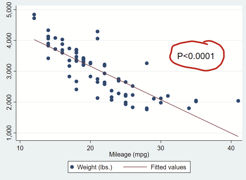
// now make a scatterplot and print out that formatted p-value
twoway ///
(scatter weight mpg) ///
(lfit weight mpg) ///
, ///
text(3500 35 "`pvalue'", size(large))
It’s handy to add text to your plots to orient your readers to specific observations in your figures. You might opt to highlight a datapoint, add percentages to bars, or say what part of a figure range is good vs. bad.
Adding text to Stata is relatively straightforward, once you get over the initial learning hump. Check out the added text help files by typing —help added_text_options— and —help textbox_options— for details.
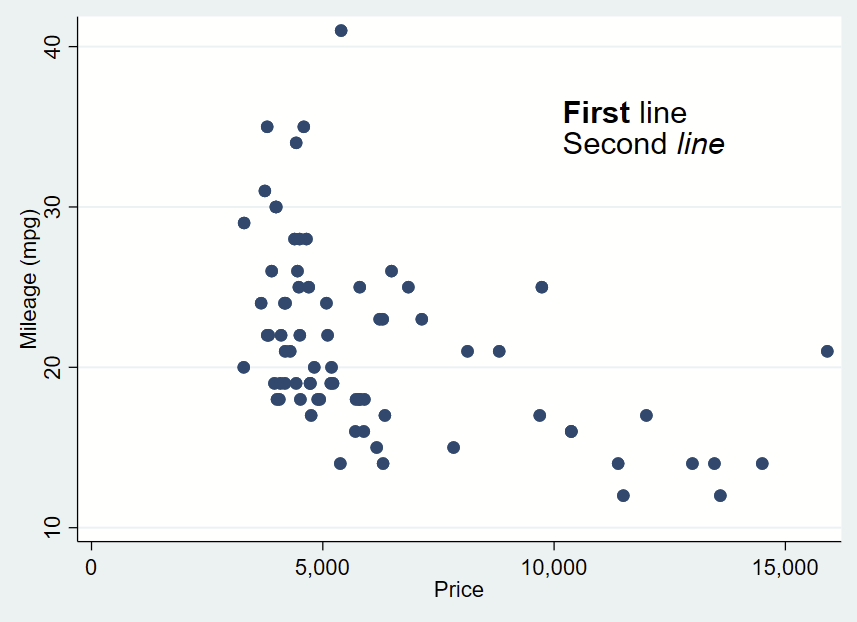
Added text syntax
First, make your figure, then add your comma, then add your syntax. Like everything(?) in Stata, the location is specified as Y then X. Then add your text in quotes (or multiple quotes in a row if you want to insert a line break). You can bold or italicize by using the it: and bf: formatting and wrapping the text you want to apply it to in brackets. Then you drop a comma, specify placement as centered (c) or cardinal directions (e.g., ne, s, w) of that text box relative to the Y,X coordinates, justification of the text as left-aligned (left), centered (center), or right-aligned (right), and size of the text (vsmall, small, medsmall, medium, medlarge, large, vlarge, huge as shown in —help textsizestyle–).
Text box without outline, playing around with bolding and italicizing:
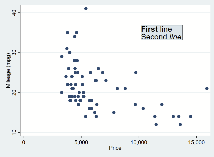
You can further customize your box by specifying options shown under —help textbox_options–. Here, I’m making a box with no fill, and a thick/dashed/red outline with fcolor (fill color, which can be “none” for blank/see-through), lcolor (outline color), lpattern (outline pattern), and lwidth (thickness of outline).
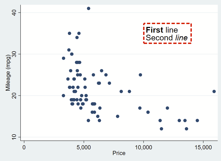
That looks pretty cool, but I’d like there to be more space between the text and the border. That’s specified with “margin”. There’s lots of complex options for this command you can read about in —help marginstyle–, but specifying “small” margin will add just a little buffer.
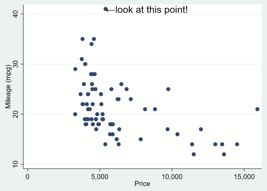
Here’s how you might use the above arrow. Here, I’ve changed the placement to “e” for “east” so the text is to the right and centered of the specified Y,X coordinates of this point (which I looked up, it’s 41,5397). I’ve dropped the box and it’s only one line. I need to manually specify the Y,X coordinates, so it’s a bit clunky still.
sysuse auto, clear
twoway ///
(scatter mpg price) ///
, ///
text(41 5397 "←look at this point!", placement(e) justification(left) size(large))
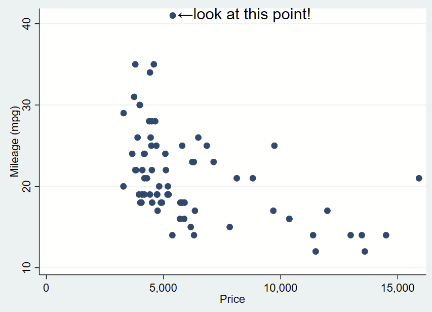
You’ll notice that the left pointing arrow is inside the point of interest. The left pointing arrow in Ariel text isn’t exactly vertically centered (that’s a quirk of Ariel). You can “nudge” the text box to the right and up by adding an offset to the Y and X coordinates. To do math on an x,y point and add an offset, you place the point in an opening tick (to the left of 1 on your keyboard) and an apostrophe, and putting an equal sign at the beginning. After a bit of trial and error, we want to add an offset of +0.3 to the Y coordinate and +200 to the X coordinate.
sysuse auto, clear
twoway ///
(scatter mpg price) ///
, ///
text(`=41+0.3' `=5397+200' "←look at this point!", placement(e) justification(left) size(large))
If we want to automate the extreme numbers on either axis, we can use the sum command to grab the maximum value aka r(max) of the Y axis and the corresponding x value for that extreme. We can make a local macro to grab that value. Since this uses local macros, you need to run all lines at once in a do file, not line by line.
sysuse auto, clear
// grab yaxis (mpg) extreme
sum mpg, d
// now look at the r-value scalars we can call.
// note that r(max) is 41 and is the maximum.
return list
// now save r(max) as a local macro
local ymax = r(max)
// now let's find the x value for that y value.
// remember that the x axis variable is "price"
sum price if mpg==`ymax', d
// now look at r-value scalars you can call.
// since there's only 1 value, the mean, min, max,
// and sum are all the same.
return list
// let's now grab the r(mean) of as a local macro
local ymax_x = r(mean)
// now you can prove that you grabbed the correct point
di "Y max =" `ymax' ", and that point is at X=" `ymax_x'
// now place those local macros in the Y and X, keeping
// the other offsets
twoway ///
(scatter mpg price) ///
, ///
text(`=`ymax'+0.3' `=`ymax_x'+200' "←look at this point!", placement(e) justification(center) size(large))
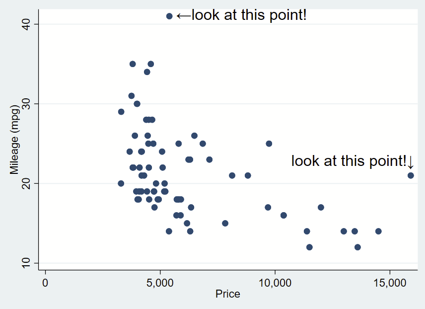
You can do the same for the x-axis extreme in the same script. for the X extreme, we’ll change the placement so it’s northwest and also tweak the Y,X coordinate offsets.
sysuse auto, clear
sum mpg, d
local ymax = r(max)
sum price if mpg==`ymax', d
local ymax_x = r(mean)
di "Y max =" `ymax' ", and that point is at X=" `ymax_x'
//
sum price, d
local xmax=r(max)
sum mpg if price==`xmax', d
local xmax_y=r(mean)
di "X max =" `xmax' ", and that point is at Y=" `xmax_y'

twoway ///
(scatter mpg price) ///
, ///
text(`=`ymax'+0.3' `=`ymax_x'+200' "←look at this point!", placement(e) justification(center) size(large)) ///
text(`=`xmax_y'+1' `=`xmax'+260' "look at this point!↓", placement(nw) justification(center) size(large))
What about adding text labels bar graphs?
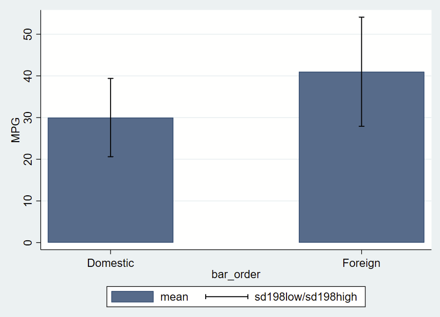
There’s a simple –graph bar– command, which isn’t terribly customizable. Here, we’ll be using the –twoway bar– bar graphs and add some fancy error bars with –twoway rcap–. The simplest way to do this is to make a new “dataset” from summary statistics in a separate frame. Frames are new in Stata 16, so if you are using an older version, this won’t work.
After making a frame with a bunch of summary statistics by group (most of which we won’t use here, but you might opt to later so we’ll keep it all there), you get this figure of mean and +/- 1.98*SD error bars.
// this has local macros so need to run from top to bottom in a do file!
// clear all frames
version 16
frames reset
sysuse auto, clear
// make a new frame called "bardata" that will store the values for bars.
frame create bardata str20 rowname n low95 high95 mean sd median iqrlow iqrhigh bar_order
//
// now grab summary statistics for foreign==0
// grab 2.5th and 95th %ile and save as local macros
// in case you might want them ever
_pctile mpg if foreign==0, percentiles(2.5 97.5)
local low95 = r(r1)
local high95= r(r2)
// now sum with detail one row
sum mpg if foreign==0, d
// post these to the new frame/bardata
// note the final row, which will be the x axis value that will correspond with bar placement
frame post bardata  ("Foreign==0") (r(N)) (r(mean)) (`low95') (`high95') (r(sd)) (r(p50)) (r(p25)) (r(p75)) (1)
//
// now repeat for foreign==1
_pctile mpg if foreign==1, percentiles(2.5 97.5)
local low95 = r(r1)
local high95= r(r2)
sum mpg if foreign==1, d
// note the final row is now 3, leaving a gap of between the prior row
frame post bardata  ("Foreign==1") (r(N)) (r(mean)) (`low95') (`high95') (r(sd)) (r(p50)) (r(p25)) (r(p75)) (3)

// now change to the frame with the summary statistics
cwf bardata
// let's make a new variable that's the mean +/- 1.98*sd
gen sd198low = mean-(sd*1.98)
gen sd198high = mean+(sd*1.98)

// now graph those data
twoway ///
(bar mean bar_order) ///
(rcap sd198low sd198high bar_order, vert lcolor(black)) ///
, ///
yla(0(10)50) ///
xla(1 "Domestic" 3 "Foreign") ///
ytitle("MPG")
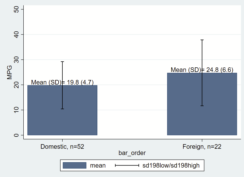
Let’s make things a bit more fancy with labels, and place a text box with the mean and SD immediately above/north of the bars, which themselves are means of MPG by group. One quirk of Stata is that when formatting printed text from stored values, you need to place the label in an opening and closing tick, put a colon, type display, then apply the formatting (e.g., %3.1f for 1 digit after the decimal) then the value you are trying to show. You’ll notice that formatting in the last two lines of the following code.
// clear all frames
version 16
frames reset
sysuse auto, clear
// make a new frame called "bardata" that will store the values for bars.
frame create bardata str20 rowname n mean low95 high95  sd median iqrlow iqrhigh bar_order
//
// now grab summary statisticis for foreign==0
// grab 2.5th and 95th %ile and save as local macros
_pctile mpg if foreign==0, percentiles(2.5 97.5)
local low95 = r(r1)
local high95= r(r2)
// now sum with detail one row
sum mpg if foreign==0, d
// post these to the new frame/bardata
// note the final row, which will be the x axis value that will correspond with bar placement
frame post bardata  ("Foreign==0") (r(N)) (r(mean)) (`low95') (`high95') (r(sd)) (r(p50)) (r(p25)) (r(p75)) (1)
//
// now repeat for foreign==1
_pctile mpg if foreign==1, percentiles(2.5 97.5)
local low95 = r(r1)
local high95= r(r2)
sum mpg if foreign==1, d
// note the final row is now 3, leaving a gap of between the prior row
frame post bardata  ("Foreign==1") (r(N)) (r(mean)) (`low95') (`high95') (r(sd)) (r(p50)) (r(p25)) (r(p75)) (3)

// now change to the frame with the summary statistics
cwf bardata
// let's make a new variable that's the mean +/- 1.98*sd
gen sd198low = mean-(sd*1.98)
gen sd198high = mean+(sd*1.98)

// let's grab the mean and SD for each group. This frame has only two
// rows of data, so we'll use the row notatition to generate a local from
// the first and second rows, with row number specified in brackets
local group0_mean = mean[1]
local group0_sd =sd[1]
local group0_n = n[1]
// print to check your work
di "for group 0, mean =" `group0_mean' ", SD=" `group0_sd' ", n=" `group0_n'
// do the other group
local group1_mean = mean[2]
local group1_sd =sd[2]
local group1_n = n[2]
// print to check your work
di "for group 1, mean =" `group1_mean' ", SD=" `group1_sd' ", n=" `group1_n'

// now graph those data
// we'll add labels for the mean and SD and also
// label the N in the xlabels
twoway ///
(bar mean bar_order) ///
(rcap sd198low sd198high bar_order, vert lcolor(black)) ///
, ///
yla(0(10)50) ///
xla(1 "Domestic, n=`group0_n'" 3 "Foreign, n=`group1_n'") ///
ytitle("MPG") ///
text(`group0_mean' 1 "Mean (SD)= `: display %3.1f `group0_mean'' (`: display %3.1f `group0_sd'')", placement(n)) ///
text(`group1_mean' 3 "Mean (SD)= `: display %3.1f `group1_mean'' (`: display %3.1f `group1_sd'')", placement(n))
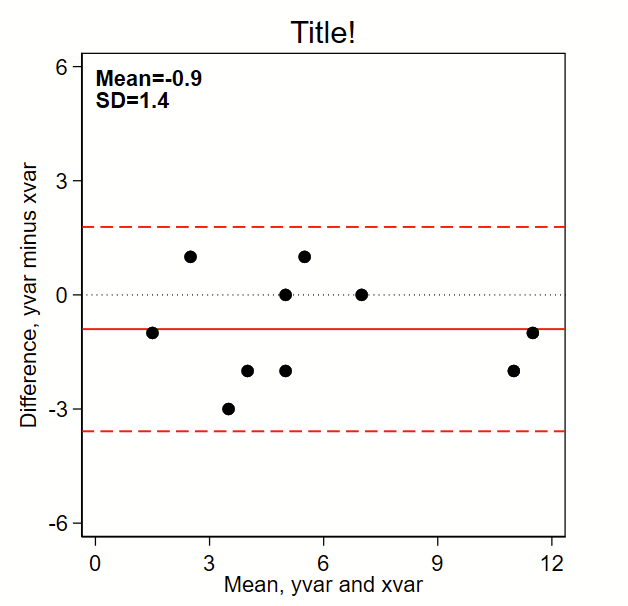
The below code outputs this Bland-Altman plot figure, which prints the mean and SD and puts a solid line for mean difference and red dotted lines for mean difference +/- 1.96*SD. (Note: the original BA paper used +/- 2*SD, but it’s reasonable to use +/-1.96*SD given it’s commonality in estimating the bounds of 95% confidence intervals of a normally-distributed plot). By the way, see the related page on making a scatterplot here, which should probably be shown alongside this figure in any publication.
Here’s the code:
// note this uses local macros so you need to run this entire thing
// top to bottom in a do file, not line by line.
//
// Step 1: input some fake data:
// Note: for comparing tests (e.g., lab tests), I make x the "gold standard"
//       test and y the investigational test
clear all

input id yvar xvar
1 2 5
2 3 5
3 6 5
4 7 7
5 3 2
6 10 12
7 1 2
8 11 12
9 4 6
10 5 5
end

// Step 2a: make difference (to go on y axis) and mean (x axis) variables
gen diff= yvar - xvar
gen mean = (yvar+xvar)/2

// Step 2b: Grab the difference (y axis) mean and sd
sum diff, d
local diffmean= r(mean)
local diffsd = r(sd)

// Step 3: graph!
set scheme s1mono // I like this scheme

twoway ///
(scatter diff mean, msymbol(O) msize(medium) mcolor(black)) ///
, ///
/// black dotted line at zero:
yline(0, lcolor(black) lpattern(dot) lwidth(medium)) ///
/// red solid line at mean:
yline(`=`diffmean'',lcolor(red) lpattern(solid) lwidth(medium)) ///
/// red dashed lines at mean +/- 1.96*sd
yline(`=`diffmean'+1.96*`diffsd''  , lcolor(red) lpattern(dash) lwidth(medium)) ///
yline(`=`diffmean'-1.96*`diffsd''  , lcolor(red) lpattern(dash) lwidth(medium)) ///
aspect(1) /// force output to be square
/// here's the text box with mean and sd,
/// you'll need to tweak the first two numbers so the y,x
/// coordinates drop the text where you want it
text(6 0 "{bf:Mean=`:di %3.1f `=`diffmean'''}" "{bf:SD=`:di %3.1f `=`diffsd'''}", placement(se) justification(left)) ///
legend(off) /// Shut off the legend
/// Now tweak the ranges of the axes to your liking.
/// I like to make them the same width. In this example, the x axis is from
/// 0 to 12 so is 12 units wide. So I set the y axis to also be
/// 12 units wide, going from -6 to +6.
xla(0(3)12) /// you'll need to tweak range for your data
yla(-6(3)6, angle(0)) /// you'll need to tweak range for your data
ytitle("Difference, yvar minus xvar") ///
xtitle("Mean, yvar and xvar") ///
title("Title!")
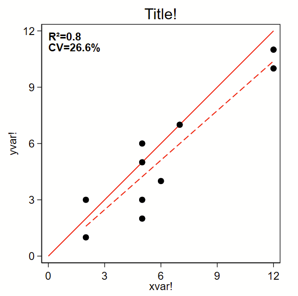
I recently had to make some scatterplots for Figure 3 of this paper. I decided to clean up the code in case it might be helpful to others.
The below code outputs a scatterplot with R-squared and %CV. I grabbed the %CV-from-a-regression code from Mehmet Mehmetoglu’s CV program. (Type –ssc install cv– to grab that one. It’s not needed for below.) By the way, you might also be interested in how to make a related Bland-Altman plot here.
Here’s the code:
// note this uses local macros so you need to run this entire thing
// top to bottom in a do file, not line by line.
//
// Step 1: input some fake data:
clear all

input id yvar xvar
1 2 5
2 3 5
3 6 5
4 7 7
5 3 2
6 10 12
7 1 2
8 11 12
9 4 6
10 5 5
end

// Step 2a: Grab the R2 from a regresssion
regress yvar xvar
local rsq = e(r2)
// Step 2b, from the same regression, calculate the percent CV
local  rmse= e(rmse)
local depvar = e(depvar)
sum `depvar' if e(sample), meanonly
local depvarmean = r(mean)
local cv = `rmse'/`depvarmean'*100

// Step 3: graph!
set scheme s1mono // I like this scheme

twoway ///
/// Line of unity, you'll need to tweak the range for your data.
/// note that 'y' and 'x' are not the same as 'yvar' and 'xvar'
/// but are instead what's required here to print the line of
/// unity:
(function y=x , range(0 12) lcolor(red) lpattern(solid) lwidth(medium)) ///
/// line of fit:
(lfit yvar xvar,  lcolor(red) lpattern(dash) lwidth(medium)) ///
/// Scatter plot dots:
(scatter yvar xvar, msymbol(O) msize(medium) mcolor(black)) ///
, ///
aspect(1) /// force output to be square
/// here's the text box with R2 and CV,
/// you'll need to tweak the first two numbers so the y,x
/// coordinates drop the text where you want it
text(12 0 "{bf:R²=`:di %3.1f `=`rsq'''}" "{bf:CV=`:di %4.1f `=`cv'''%}", placement(se) justification(left)) ///
legend(off) /// Shut off the legend
yla(0(3)12, angle(0)) /// you'll need to tweak range for your data
xla(0(3)12) /// you'll need to tweak range for your data
ytitle("yvar!") ///
xtitle("xvar!") ///
title("Title!")
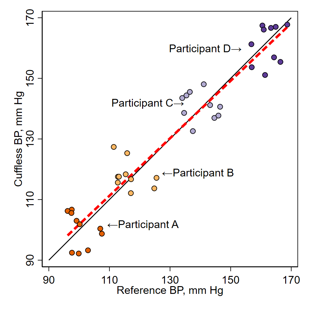
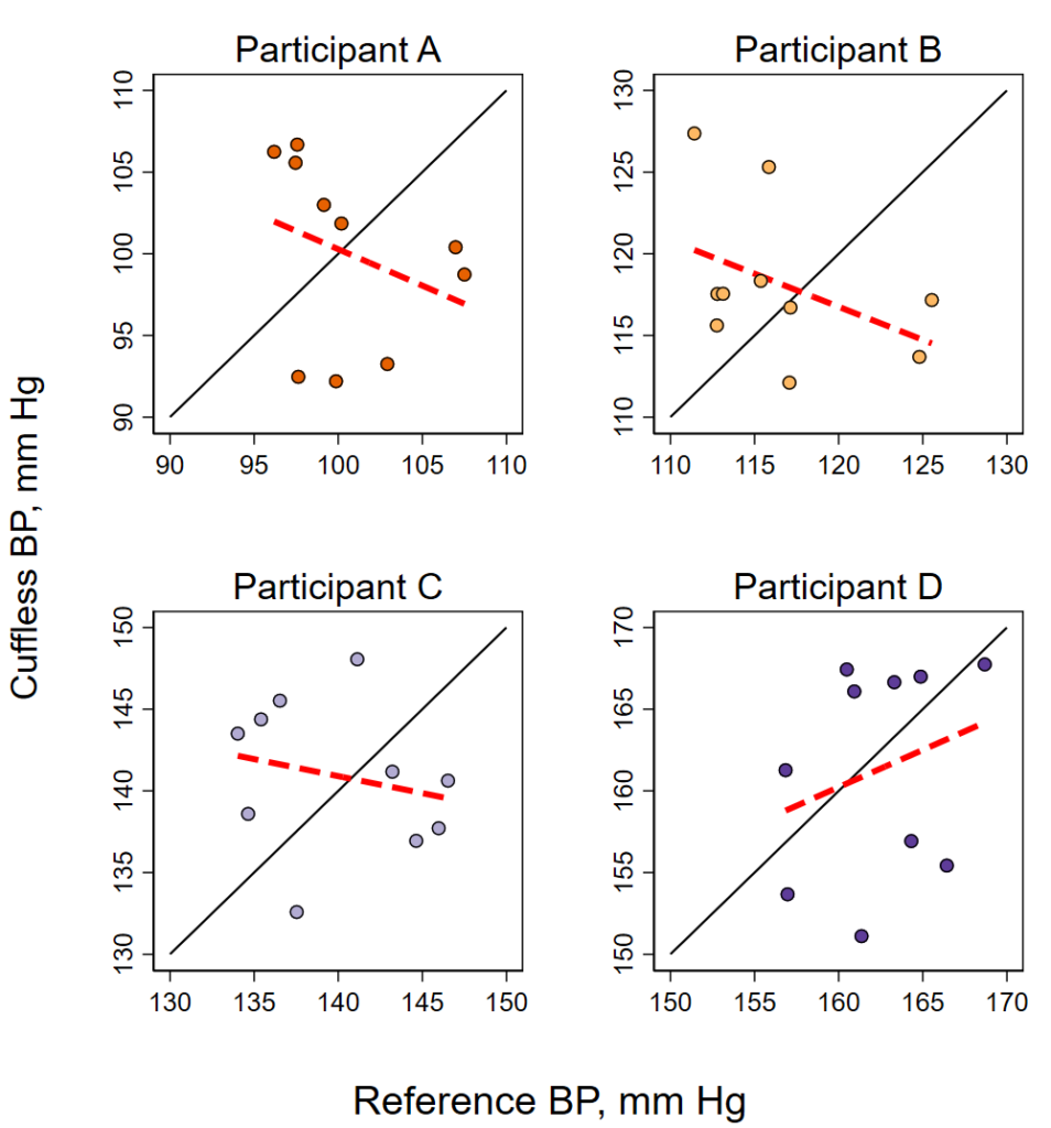
I recently made these two figures with a Stata do file that (A) generates some fake data, (B) plots the data overall with a fitted line, (C) plots each participant individually with fitted line, and (D) merges these four individual plots into one overall plot. One tricky piece of this was to get the –graph combine– command to get the four figures to be square, I had to fiddle with the –ysize– to get them to be square. I had originally tried using the –aspect– option, but it builds in lots of white space to between the figures. this way seemed to work.
Here’s the Stata code to make the above figures.
************************
*****clear data/graphs**
****set graph schemes***
************************
clear
graph drop _all
set scheme s1mono

************************
*****generate data******
************************
set seed 8675309
// generate 40 random values
set obs 40
//...called x and y that range from - to +9
gen y = runiform(-9,9)
gen x = runiform(-9,9)
// now make an indicator for each grouping of 10
gen n =.
replace n= 1 if _n>=0 & _n<=10
replace n= 2 if _n>10 & _n<=20
replace n= 3 if _n>20 & _n<=30
replace n= 4 if _n>30 & _n<=40
// now for each successive 10 rows, add 100, 120, 140, and 160
replace y = y+100 if n==1
replace x = x+100 if n==1

replace y = y+120 if n==2
replace x= x+120 if n==2

replace y= y+140 if n==3
replace x= x+140 if n==3

replace y= y+160 if n==4
replace x= x+160 if n==4
************************
*****single figure******
************************
twoway ///
/// line of unity (45 degree line):
(function y = x, ra(90 170) clpat(solid) clwidth(medium) clcolor(black)) ///
/// line of fit:
(lfit y x, lcolor(red) lpattern(dash) lwidth(thick)) ///
/// dots for each group, using colors from colorbrewer2
(scatter y x if n==1, mcolor("230 97 1") msymbol(O) mlcolor(black)) ///
(scatter y x if n==2, mcolor("253 184 99") msymbol(O) mlcolor(black)) ///
(scatter y x if n==3, mcolor("178 171 210") msymbol(O) mlcolor(black)) ///
(scatter y x if n==4, mcolor("94 60 153") msymbol(O) mlcolor(black)) ///
, ///
/// force size:
ysize(4) xsize(4) ///
/// axis titles and rows:
xtitle("Reference BP, mm Hg") ///
ytitle("Cuffless BP, mm Hg") ///
xla(90(20)170) ///
yla(90(20)170) ///
legend(off) ///
/// labels:
text(102 109 "←Participant A", placement(e)) ///
text(119 127 "←Participant B", placement(e)) ///
text(142 135 "Participant C→", placement(w)) ///
text(160 154 "Participant D→", placement(w))
/// export figure:
graph export figure1av2.png, replace width(1000)


************************
***four-piece figures***
*****to merge***********
************************
twoway ///
(function y = x if n==1, ra(90 110) clpat(solid) clwidth(medium) clcolor(black)) ///
(lfit y x if n==1, lcolor(red) lpattern(dash) lwidth(thick)) ///
(scatter y x if n==1, mcolor("230 97 1") msymbol(O) mlcolor(black)) ///
, ///
title("Participant A") ///
xtitle(" ") ///
ytitle(" ") ///
yla(90(5)110) ///
xla(90(5)110) ///
legend(off) ///
name(figure1b1)

twoway ///
(function y = x if n==2, ra(110 130) clpat(solid) clwidth(medium) clcolor(black)) ///
(lfit y x if n==2, lcolor(red) lpattern(dash) lwidth(thick)) ///
(scatter y x if n==2, mcolor("253 184 99") msymbol(O) mlcolor(black)) ///
, ///
title("Participant B") ///
xtitle(" ") ///
ytitle(" ") ///
yla(110(5)130) ///
xla(110(5)130) ///
legend(off) ///
name(figure1b2)

twoway ///
(function y = x if n==3, ra(130 150) clpat(solid) clwidth(medium) clcolor(black)) ///
(lfit y x if n==3, lcolor(red) lpattern(dash) lwidth(thick)) ///
(scatter y x if n==3, mcolor("178 171 210") msymbol(O) mlcolor(black)) ///
, ///
title("Participant C") ///
xtitle(" ") ///
ytitle(" ") ///
yla(130(5)150) ///
xla(130(5)150) ///
legend(off) ///
name(figure1b3)

twoway ///
(function y = x if n==4, ra(150 170) clpat(solid) clwidth(medium) clcolor(black)) ///
(lfit y x if n==4, lcolor(red) lpattern(dash) lwidth(thick)) ///
(scatter y x if n==4, mcolor("94 60 153") msymbol(O) mlcolor(black)) ///
, ///
title("Participant D") ///
xtitle(" ") ///
ytitle(" ") ///
yla(150(5)170) ///
xla(150(5)170) ///
legend(off) ///
name(figure1b4)

***********************
***combine figures*****
***********************
graph combine figure1b1 figure1b2 figure1b3 figure1b4 /*figure1b5*/, ///
b1title("Reference BP, mm Hg") ///
l1title("Cuffless BP, mm Hg") ///
/// this forces the four scatterplots to be the same height/width
/// details here:
/// https://www.stata.com/statalist/archive/2013-07/msg00842.html
cols(2) iscale(.7273) ysize(5.9) graphregion(margin(zero))

/// export to figure
graph export figure1bv2.png, replace width(1000)
Stata 16 introduced the new Frames functionality, which allows multiple datasets to be stored in memory, with each dataset stored in its own “Frame”. This allows for dynamic manipulation of multiple datasets across multiple Frames. Stata is still simplest to use when manipulating a single dataset (or, frame). So, Stata users will probably be interested in building a single dataset/Frame for a specific analysis that is built from variables taken from multiple datasets/Frames.
One handy application of Frames is to import non-Stata datasets as separate frames and combine them (really, merge) into a single analytical dataset/Frame. Before using Frames, I had previously imported non-Stata datasets, saved them locally, then merged them 1 by 1. With Frames, you just import each dataset into its own Frame, and “merge” them directly, skipping the intermediate “save as Stata dta file” step.
Here’s my approach to building a single analytical dataset from multiple imported datasets, with frames. We’ll do this with NHANES data. This is a modification of the code on this post.
Step 1: Drop (reset) all frames, create new ones to import the new datasets, and run commands within each new frame to import NHANES/SAS datasets.
// Here's the NHANES website, FYI:
// https://wwwn.cdc.gov/nchs/nhanes/default.aspx
//
// drop all frames from memory. This will delete all unsaved data so be careful!!
frames reset
//
// make a blank frame called "DEMO_F"
// you could type "frame create" or the brief synonym "mkf" for
// "make frame"
mkf DEMO_F
// ...Then run the sas import command within it, grabbing it from the CDC website.
// Since this command needs to be run from within the DEMO_F frame,
// we can tell Stata to run the command from that frame without
// actually changing to it using the "frame [name]:" prefix
frame DEMO_F: import sasxport5 "https://wwwn.cdc.gov/Nchs/Nhanes/2009-2010/DEMO_F.XPT", clear
//
// ditto for the "BPQ_F" and "KIQ_U_F" datasets.
mkf BPQ_F
frame BPQ_F: import sasxport5 "https://wwwn.cdc.gov/Nchs/Nhanes/2009-2010/BPQ_F.XPT", clear
//
mkf KIQ_U_F
frame KIQ_U_F: import sasxport5 "https://wwwn.cdc.gov/Nchs/Nhanes/2009-2010/KIQ_U_F.XPT", clear
//
// let's see a list of current frames:
frames dir
//
// Which frame are you using though?
// pwf is present working frame, or the current one in use.
pwf
// You'll see that the pwf if "default".
Step 2: Create an “analytical” frame that will contain the data you need to complete your analysis, and copy the variable that links all of your data to this frame. Also switch to that new analytical frame.
// The "linking" variable in this dataset is called "seqn", which
// we will copy ("put") from the DEMO_F frame.
// (Your file might have a linking variable called "id".)
// This creates a new frame called "analytical" and also moves the "seqn"
// variable from DEMO_F to the new analytical frame in one line.
frame DEMO_F: frame put seqn, into(analytical)
//
// see current list of frames and present working frame:
frames dir
pwf
// Now change from the default frame to the new analytical one.
// You can change frames with "cwf" for "change working frame".
cwf analytical
Step 3: Now that you are are in the new analytical frame, link all of your frames using the “linking” variable (“seqn” here).
// use the "frlink" command to link frames. This can be 1:1 linking or 1:m.
//
// remember that your cwf should be analytical right now.
//
frlink 1:1 seqn, frame(DEMO_F)
frlink 1:1 seqn, frame(BPQ_F)
frlink 1:1 seqn, frame(KIQ_U_F)
//
// You are still within the "analytical" frame, but now your frames are all
// linked or connected to each other.
// if you look at your dataset with the --browse-- command, you'll see there
// are now new DEMO_F, BPQ_F, and KIQ_U_F variables. These are the "rows" for
// linked IDs in those other frames, so Stata knows where to look for
// variables in those other frames.
Step 4: “Get” the specific variables you want from each frame. This is how you merge individual variables from multiple frames.
// from my NHANES post, we need to grab weighting variables from DEMO_F
// and a BP variable from BPQ_F. Just for kicks, we'll also grab self-
// reported "weak kidneys" from KIQ_U_F.
//
// remember that your cwf should be analytical right now.
//
frget wtint2yr wtmec2yr sdmvpsu sdmvstra, from(DEMO_F)
frget bpq020, from(BPQ_F)
frget kiq022, from(KIQ_U_F)
//
// now you have a nice merged database!
Step 5 (optional): If you are satisfied with your analytical dataset and no longer need the other frames, you can now drop the “linking” variables from the analytical dataset, save your analytical dataset, clear your frames, and reopen your analytical dataset
// You can save this analytical frame as a Stata
// dataset now if you are done manipulating the other frames.
//
// You might opt to drop the new linking variables prior to saving
// for simplicity.
drop DEMO_F BPQ_F KIQ_U_F
//
// Stata's "save" command won't save other frames as FYI, just the pwf.
// But in this example, we are done with other frames.
save analytical.dta, replace
//
// Drop all other frames so you don't get an annoying pop-up
// about unsaved frames in memory.
// Be careful! This will drop all data from memory!!
frames reset
//
// now reopen your previously saved analytical dataset.
use analytical.dta, clear
Bonus: Appending frames
You might need to append frames. There are some details here about how to do this. I’m using the –fframeappend– command by Jürgen Wiemers.
// install fframeappend, only need to do once:
ssc install fframeappend
// change to the frame you want to append all of your data to,
// in this example it's called "appended"
// you'll have to use "mkf appended" if you don't already have one
// called that.
cwf appended
//now append your frame "a" to the current open frame
fframeappend, using(a)
// now repeat using frame "b" to the current open frame
fframeappend, using(b)
Bonus: Here’s steps 1-4 in a single loop using global macros
For advanced users: Here’s a loop and some global macros that is adaptable to downloading several years. NHANES uses different letters for files from different years, the 2009-2010 one uses “F”.
frames reset
global url "https://wwwn.cdc.gov/Nchs/Nhanes/"
global F "2009-2010/"
global files DEMO BPQ KIQ_U

foreach x in F {
	foreach y in $files {
		mkf `y'_`x'
		frame `y'_`x': import sasxport5 "${url}${`x'}`y'_`x'.xpt"
	}
frame DEMO_`x': frame put seqn, into(analytical_`x')
cwf analytical_`x'
	foreach y in $files {
		frlink 1:1 seqn, frame(`y'_`x')
	}
	frget wtint2yr wtmec2yr sdmvpsu sdmvstra, from(DEMO_`x')
	frget bpq020, from(BPQ_`x')
	frget kiq022, from(KIQ_U_`x')
}
frames dir
pwf
Here’s the same as above, but just for a single year.
frames reset
global dir "https://wwwn.cdc.gov/Nchs/Nhanes/2009-2010/"
global files DEMO_F BPQ_F KIQ_U_F

foreach y in $files {
	mkf `y'
	frame `y': import sasxport5 "${dir}`y'.xpt"
}
frame DEMO_F: frame put seqn, into(analytical)
cwf analytical
foreach y in $files {
	frlink 1:1 seqn, frame(`y')
}
frget wtint2yr wtmec2yr sdmvpsu sdmvstra, from(DEMO_F)
frget bpq020, from(BPQ_F)
frget kiq022, from(KIQ_U_F)
frames dir
pwf
Mediation is a commonly-used tool in epidemiology. Inverse odds ratio-weighted (IORW) mediation was described in 2013 by Eric J. Tchetgen Tchetgen in this publication. It’s a robust mediation technique that can be used in many sorts of analyses, including logistic regression, modified Poisson regression, etc. It is also considered valid if there is an observed exposure*mediator interaction on the outcome.
There have been a handful of publications that describe the implementation of IORW (and its cousin inverse odds weighting, or IOW) in Stata, including this 2015 AJE paper by Quynh C Nguyen and this 2019 BMJ open paper by Muhammad Zakir Hossin (see the supplements of each for actual code). I recently had to implement this in a REGARDS project using a binary mediation variable and wanted to post my code here to simplify things. The code here is designed for binary exposures and not continuous exposures. Check out the Nguyen paper above if you need to modify the following code to run IOW instead of IOWR, or if you are using a continuous mediation variable, rather than a binary one.
A huge thank you to Charlie Nicoli MD, Leann Long PhD, and Boyi Guo (almost) PhD who helped clarify implementation pieces. Also, Charlie wrote about 90% of this code so it’s really his work. I mostly cleaned it up, and clarified the approach as integrated in the examples from Drs. Nguyen and Hossin from the papers above.
IORW using pweight data (see below for unweighted version)
The particular analysis I was running uses pweighting. This code won’t work in data that doesn’t use weighting. This uses modified Poisson regression implemented as GLMs. These can be swapped out for other models as needed. You will have to modify this script if you are using 1. a continuous exposure, 2. more than 1 mediator, 3. a different weighting scheme, or 4. IOW instead of IORW. See the supplement in the above Nguyen paper on how to modify this code for those changes.
*************************************************
// this HEADER is all you should have to change
// to get this to run as weighted data with binary
// exposure using IORW. (Although you'll probably
// have to adjust the svyset commands in the
// program below to work in your dataset, in all
// actuality)
*************************************************
// BEGIN HEADER
//
// Directory of your dataset. You might need to
// include the entire file location (eg "c:/user/ ...")
// My file is located in my working directory so I just list
// a name here. Alternatively, can put URL for public datasets.
global file "myfile.dta"
//
// Pick a title for the table that will output at the end.
// This is just to help you stay organized if you are running
// a few of these in a row.
global title "my cool analysis, model 1"
//
// Components of the regression model. Outcome is binary,
// the exposure (sometimes called "dependent variable" or
// "treatment") is also binary. This code would need to be modified
// for a continuous exposure variable. See details in Step 2.
global outcome mi_incident
global exposure smoking
global covariates age sex
global mediator c.biomarker
global ifstatement if mi_prevalent==0 & biomarker<. & mi_incident <.
//
// Components of weighting to go into "svyset" command.
// You might have
global samplingweight mysamplingweightvar
global id id_num // ID for your participants
global strata mystratavar
//
// Now pick number of bootstraps. Aim for 1000 when you are actually
// running this, but when debugging, start with 50.
global bootcount 50
// and set a seed.
global seed 8675309
// END HEADER
*************************************************
//
//
//
// Load your dataset.
use "${file}", clear
//
// Drop then make a program.
capture program drop iorw_weighted
program iorw_weighted, rclass
// drop all variables that will be generated below.
capture drop predprob
capture drop inverseoddsratio
capture drop weight_iorw
//
*Step 1: svyset data since your dataset is weighted. If your dataset
// does NOT require weighting for its analysis, do not use this program.
svyset ${id}, strata(${strata}) weight(${samplingweight}) vce(linearized) singleunit(certainty)
//
*Step 2: Run the exposure model, which regresses the exposure on the
// mediator & covariates. In this example, the exposure is binary so we are
// using logistic regression (logit). If the exposure is a normally-distributed
// continuous variable, use linear regression instead.
svy linearized, subpop(${ifstatement}): logit ${exposure} ${mediator} ${covariates}
//
// Now grab the beta coefficient for mediator. We'll need that to generate
// the IORW weights.
scalar med_beta=e(b)[1,1]
//
*Step 3: Generate predicted probability and create inverse odds ratio and its
// weight.
predict predprob, p
gen inverseoddsratio = 1/(exp(med_beta*${mediator}))
//
// Calculate inverse odds ratio weights.  Since our dataset uses sampling
// weights, we need to multiply the dataset's weights times the IORW for the
// exposure group. This step is fundamentally different for non-weighted
// datasets.
// Also note that this is for binary exposures, need to revise
// this code for continuous exposures.
gen weight_iorw = ${samplingweight} if ${exposure}==0
replace weight_iorw = inverseoddsratio*${samplingweight} if ${exposure}==1
//
*Step 4: TOTAL EFFECTS (ie no mediator) without IORW weighting yet.
// (same as direct effect, but without the IORW)
svyset ${id}, strata(${strata}) weight(${samplingweight}) vce(linearized) singleunit(certainty)
svy linearized, subpop(${ifstatement}): glm ${outcome} ${exposure} ${covariates}, family(poisson) link(log)
matrix bb_total= e(b)
scalar b_total=bb_total[1,1]
return scalar b_total=bb_total[1,1]
//
*Step 5: DIRECT EFFECTS; using IORW weights instead of the weighting that
// is used typically in your analysis.
svyset ${id}, strata(${strata}) weight(weight_iorw) vce(linearized) singleunit(certainty)
svy linearized, subpop(${ifstatement}): glm ${outcome} ${exposure} ${covariates}, family(poisson) link(log)
matrix bb_direct=e(b)
scalar b_direct=bb_direct[1,1]
return scalar b_direct=bb_direct[1,1]
//
*Step 6: INDIRECT EFFECTS
// indirect effect = total effect - direct effects
scalar b_indirect=b_total-b_direct
return scalar b_indirect=b_total-b_direct
//scalar expb_indirect=exp(scalar(b_indirect))
//return scalar expb_indirect=exp(scalar(b_indirect))
//
*Step 7: calculate % mediation
scalar define percmed = ((b_total-b_direct)/b_total)*100
// since indirect is total minus direct, above is the same as saying:
// scalar define percmed = (b_indirect)/(b_total)*100
return scalar percmed = ((b_total-b_direct)/b_total)*100
//
// now end the program.
end
//
*Step 8: Now run the above bootstraping program
bootstrap r(b_total) r(b_direct) r(b_indirect) r(percmed), seed(${seed}) reps(${bootcount}): iorw_weighted
matrix rtablebeta=r(table) // this is the beta coefficients
matrix rtableci=e(ci_percentile) // this is the 95% confidence intervals using the "percentiles" (ie 2.5th and 97.5th percentiles) rather than the default normal distribution method in stata. The rational for using percentiles rather than normal distribution is found in the 4th paragraph of the "analyses" section here (by refs 37 & 38): https://bmjopen.bmj.com/content/9/6/e026258.long
//
// Just in case you are curious, here are the the ranges of the 95% CI,
// realize that _bs_1 through _bs_3 need to be exponentiated:
estat bootstrap, all // percentiles is "(P)", normal is "(N)"
//
// Here's a script that will display your beta coefficients in
// a clean manner, exponentiating them when required.
quietly {
noisily di "${title} (bootstrap count=" e(N_reps) ")*"
noisily di _col(15) "Beta" _col(25) "95% low" _col(35) "95% high" _col(50) "Together"
local beta1 = exp(rtablebeta[1,1])
local low951 = exp(rtableci[1,1])
local high951 = exp(rtableci[2,1])
noisily di "Total" _col(15) %4.2f `beta1' _col(25) %4.2f `low951' _col(35) %4.2f `high951' _col(50) %4.2f `beta1' " (" %4.2f `low951' ", " %4.2f `high951' ")"
local beta2 = exp(rtablebeta[1,2])
local low952 = exp(rtableci[1,2])
local high952 = exp(rtableci[2,2])
noisily di "Direct" _col(15) %4.2f `beta2' _col(25) %4.2f `low952' _col(35) %4.2f `high952' _col(50) %4.2f `beta2' " (" %4.2f `low952' ", " %4.2f `high952' ")"
local beta3 = exp(rtablebeta[1,3])
local low953 = exp(rtableci[1,3])
local high953 = exp(rtableci[2,3])
noisily di "Indirect" _col(15) %4.2f `beta3' _col(25) %4.2f `low953' _col(35) %4.2f `high953' _col(50) %4.2f `beta3' " (" %4.2f `low953' ", " %4.2f `high953' ")"
local beta4 = (rtablebeta[1,4])
local low954 = (rtableci[1,4])
local high954 = (rtableci[2,4])
noisily di "% mediation" _col(15) %4.2f `beta4' "%" _col(25) %4.2f `low954' "%"_col(35) %4.2f  `high954' "%" _col(50) %4.2f `beta4' "% (" %4.2f `low954' "%, " %4.2f `high954' "%)"
noisily di "*Confidence intervals use 2.5th and 97.5th percentiles"
noisily di " rather than default normal distribution in Stata."
noisily di " "
}
// the end.
IORW for datasets that don’t use weighting (probably the one you are looking for)
Here is the code above, except without consideration of weighting in the overall dataset. (Obviously, IORW uses weighting itself.) This uses modified Poisson regression implemented as GLMs. These can be swapped out for other models as needed. You will have to modify this script if you are using 1. a continuous exposure, 2. more than 1 mediator, 3. a different weighting scheme, or 4. IOW instead of IORW. See the supplement in the above Nguyen paper on how to modify this code for those changes.
*************************************************
// this HEADER is all you should have to change
// to get this to run as weighted data with binary
// exposure using IORW.
*************************************************
// BEGIN HEADER
//
// Directory of your dataset. You might need to
// include the entire file location (eg "c:/user/ ...")
// My file is located in my working directory so I just list
// a name here. Alternatively, can put URL for public datasets.
global file "myfile.dta"
//
// Pick a title for the table that will output at the end.
// This is just to help you stay organized if you are running
// a few of these in a row.
global title "my cool analysis, model 1"
// Components of the regression model. Outcome is binary,
// the exposure (sometimes called "dependent variable" or
// "treatment") is also binary. This code would need to be modified
// for a continuous exposure variable. See details in Step 1.
global outcome  mi_incident
global exposure smoking
global covariates age sex
global mediator c.biomarker
global ifstatement if mi_prevalent==0 & biomarker<. & mi_incident <.
//
// Now pick number of bootstraps. Aim for 1000 when you are actually
// running this, but when debugging, start with 50.
global bootcount 50
// and set a seed.
global seed 8675309
// END HEADER
*************************************************
//
//
//
// Load your dataset.
use "${file}", clear
//
// Drop then make a program.
capture program drop iorw
program iorw, rclass
// drop all variables that will be generated below.
capture drop predprob
capture drop inverseoddsratio
capture drop weight_iorw
//
//
*Step 1: Run the exposure model, which regresses the exposure on the
// mediator & covariates. In this example, the exposure is binary so we are
// using logistic regression (logit). If the exposure is a normally-distributed
// continuous variable, use linear regression instead.
logit ${exposure} ${mediator} ${covariates} ${ifstatement}
//
// Now grab the beta coefficient for mediator. We'll need that to generate
// the IORW weights.
scalar med_beta=e(b)[1,1]
//
*Step 2: Generate predicted probability and create inverse odds ratio and its
// weight.
predict predprob, p
gen inverseoddsratio = 1/(exp(med_beta*${mediator}))
//
// Calculate inverse odds ratio weights.
// Also note that this is for binary exposures, need to revise
// this code for continuous exposures.
gen weight_iorw = 1 if ${exposure}==0
replace weight_iorw = inverseoddsratio if ${exposure}==1
//
*Step 3: TOTAL EFFECTS (ie no mediator) without IORW weighting yet. (same as direct effect, but without the IORW)
glm ${outcome} ${exposure} ${covariates} ${ifstatement}, family(poisson) link(log) vce(robust)
matrix bb_total= e(b)
scalar b_total=bb_total[1,1]
return scalar b_total=bb_total[1,1]
//
*Step 4: DIRECT EFFECTS; using IORW weights
glm ${outcome} ${exposure} ${covariates} ${ifstatement} [pweight=weight_iorw], family(poisson) link(log) vce(robust)
matrix bb_direct=e(b)
scalar b_direct=bb_direct[1,1]
return scalar b_direct=bb_direct[1,1]
//
*Step 5: INDIRECT EFFECTS
// indirect effect = total effect - direct effects
scalar b_indirect=b_total-b_direct
return scalar b_indirect=b_total-b_direct
//scalar expb_indirect=exp(scalar(b_indirect))
//return scalar expb_indirect=exp(scalar(b_indirect))
//
*Step 6: calculate % mediation
scalar define percmed = ((b_total-b_direct)/b_total)*100
// since indirect is total minus direct, above is the same as saying:
// scalar define percmed = (b_indirect)/(b_total)*100
return scalar percmed = ((b_total-b_direct)/b_total)*100
//
// now end the program.
end
//
*Step 7: Now run the above bootstraping program
bootstrap r(b_total) r(b_direct) r(b_indirect) r(percmed), seed(${seed}) reps(${bootcount}): iorw
matrix rtablebeta=r(table) // this is the beta coefficients
matrix rtableci=e(ci_percentile) // this is the 95% confidence intervals using the "percentiles" (ie 2.5th and 97.5th percentiles) rather than the default normal distribution method in stata. The rational for using percentiles rather than normal distribution is found in the 4th paragraph of the "analyses" section here (by refs 37 & 38): https://bmjopen.bmj.com/content/9/6/e026258.long
//
// Just in case you are curious, here are the the ranges of the 95% CI,
// realize that _bs_1 through _bs_3 need to be exponentiated:
estat bootstrap, all // percentiles is "(P)", normal is "(N)"
//
// Here's a script that will display your beta coefficients in
// a clean manner, exponentiating them when required.
quietly {
noisily di "${title} (bootstrap count=" e(N_reps) ")*"
noisily di _col(15) "Beta" _col(25) "95% low" _col(35) "95% high" _col(50) "Together"
local beta1 = exp(rtablebeta[1,1])
local low951 = exp(rtableci[1,1])
local high951 = exp(rtableci[2,1])
noisily di "Total" _col(15) %4.2f `beta1' _col(25) %4.2f `low951' _col(35) %4.2f `high951' _col(50) %4.2f `beta1' " (" %4.2f `low951' ", " %4.2f `high951' ")"
local beta2 = exp(rtablebeta[1,2])
local low952 = exp(rtableci[1,2])
local high952 = exp(rtableci[2,2])
noisily di "Direct" _col(15) %4.2f `beta2' _col(25) %4.2f `low952' _col(35) %4.2f `high952' _col(50) %4.2f `beta2' " (" %4.2f `low952' ", " %4.2f `high952' ")"
local beta3 = exp(rtablebeta[1,3])
local low953 = exp(rtableci[1,3])
local high953 = exp(rtableci[2,3])
noisily di "Indirect" _col(15) %4.2f `beta3' _col(25) %4.2f `low953' _col(35) %4.2f `high953' _col(50) %4.2f `beta3' " (" %4.2f `low953' ", " %4.2f `high953' ")"
local beta4 = (rtablebeta[1,4])
local low954 = (rtableci[1,4])
local high954 = (rtableci[2,4])
noisily di "% mediation" _col(15) %4.2f `beta4' "%" _col(25) %4.2f `low954' "%"_col(35) %4.2f  `high954' "%"  _col(50) %4.2f `beta4' " (" %4.2f `low954' ", " %4.2f `high954' ")"
noisily di "*Confidence intervals use 2.5th and 97.5th percentiles"
noisily di " rather than default normal distribution in Stata."
noisily di " "
}
// the end.
If you are looking to automate the printing of values from macros/regressions or whatnot on your figures, make sure to check out this post.
I love Stata’s macro functionality. It allows you to grab information from r- or e-level data after executing a Stata command then calling that back later. (Local macros are temporary, global macros are more persistent.) This is particularly useful when generating summary statistics collected in macros after the –sum– command, or displaying a subset of components from a regression, such as the beta coefficient and 95% confidence intervals, or P-values (details on how to manipulate regression function results with macros are here).
One problem in using macros is that raw r- or e-level data are really long and not amenable to output in tables for publication without formatting. I’ve hadn’t previously been able to apply formatting (eg %4.2f) while generating macros, outside of applying the “round” command. (I don’t like the round command because it’s tricky to code in a program for reasons I won’t get into.) Instead, I have applied the number formatting when displaying the macro. That creates issues when generating string output from numerical macros, since my prior strategy of applying numerical formatting (eg %4.2f) didn’t work when displaying a numerical macro in a string (i.e., embedding it within quotations). Instead, I wanted to apply the format while also generating the macro itself.
It turns out that not only can you apply formatting while generating a macro with the “: display” subcommand, you can also trim extra spaces from the generated macro at the same time. (Note that the “trim” command has been replaced by “strltrim” and a lot of other related commands that you can find in –help string functions–.) As a bonus, it turns out that you can also apply formatting (e.g., %4.2f) of a macro when displaying within a string using the “: display” subcommand strategically surrounded by opening and closing tick marks.
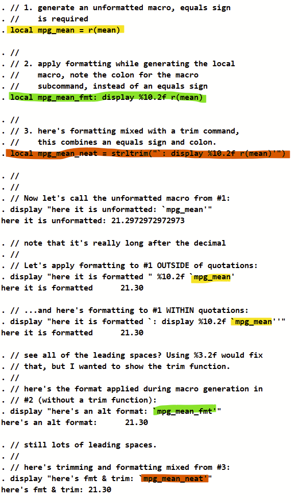
Here’s a demo script of what I’m getting at.
(Note: I strongly recommend against formatting/rounding/reducing precision of any macros that you are generating if you will later do math on them. Formatting during generation of macros is only useful for macros intended to be displayed later on.)
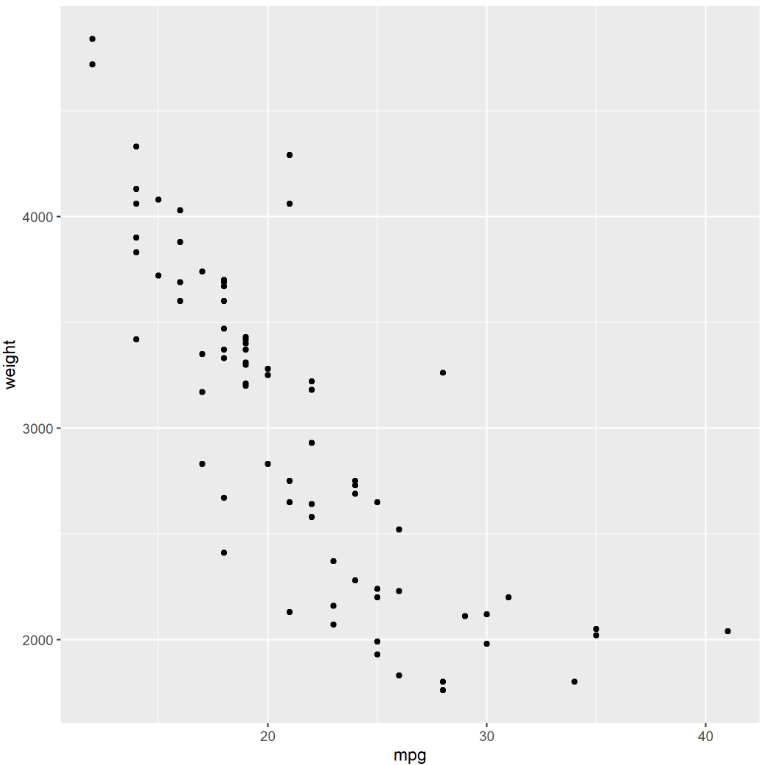
sysuse auto, clear
sum mpg
//
// 1. generate an unformatted macro, equals sign
//    is required
local mpg_mean = r(mean)
//
// 2. apply formatting while generating the local
//    macro, note the colon for the macro
//    subcommand, instead of an equals sign
local mpg_mean_fmt: display %10.2f r(mean)
//
// 3. here's formatting mixed with a trim command,
//    this combines an equals sign and colon.
local mpg_mean_neat = strltrim("`: display %10.2f r(mean)'")
//
//
// Now let's call the unformatted macro from #1:
display "here it is unformatted: `mpg_mean'"
// note that it's really long after the decimal
//
// Let's apply formatting to #1 OUTSIDE of quotations:
display "here it is formatted " %10.2f `mpg_mean'
// ...and here's formatting to #1 WITHIN quotations:
display "here it is formatted `: display %10.2f `mpg_mean''"
// see all of the leading spaces? Using %3.2f would fix
// that, but I wanted to show the trim function.
//
// here's the format applied during macro generation in
// #2 (without a trim function):
display "here's an alt format: `mpg_mean_fmt'"
// still lots of leading spaces.
//
// here's trimming and formatting mixed from #3:
display "here's fmt & trim: `mpg_mean_neat'"
// Bingo!
Stata allows the labeling of variables and also the individual values of categorical or ordinal variable values. For example, in the –sysuse auto– database, “foreign” is labeled as “Car origin”, 0 is “Domestic”, and 1 is “Foreign”. It isn’t terribly intuitive to extract the variable label of foreign (here, “Car origin”) or the labels from the categorical values (here, “Domestic” and “Foreign”).
Here’s a script that you might find helpful to extract these labels and save them as macros that can later be called back. This example generates a second string variable that applies those labels. I use this sort of code to automate the labeling of figures with the value labels, but this is a pretty simple example for now.
Remember to run the entire script from top to bottom or else Stata might drop your macros. Good luck!
sysuse auto, clear
// Note: saving variable label details at
//       --help macro--, under "Macro functions
//       for extracting data attributes"
//
// 1. Extract the label for the variable itself.
//    If we look at the --codebook-- for the
//    variable "foreign", we see...
//
codebook foreign
//
//    ...that the label for "foreign" is "Car
//    origin" (see it in the top right of
//    the output).  Here's how we grab the
//    label of "foreign", save it as a macro,
//    and print it.
//
local foreign_lab: variable label foreign
di "`foreign_lab'"
//
// 2. Extract the label for the values of the variable.
//    If we look at --codebook-- again for "foreign",
//    we see...
//
codebook foreign
//
//    ...that 0 is "Domestic" and 1 is "Foreign".
//    Here's how to grab those labels, save macros,
//    and print them
//
local foreign_vallab_0: label (foreign) 0
local foreign_vallab_1: label (foreign) 1
di "The label of `foreign_lab' 0 is `foreign_vallab_0' and 1 is `foreign_vallab_1'"
//
// 3. Now you can make a variable for the value labels.
//
gen strL foreign_vallab = "" // this makes a string
replace foreign_vallab="`foreign_vallab_0'" if foreign==0
replace foreign_vallab="`foreign_vallab_1'" if foreign==1
//
// 4. You can also label this new string variable
//    using the label from #1
//
label variable foreign_vallab "`foreign_lab' as string"
//
// BONUS: You can automate this with a loop, using
//    --levelsof-- to extract options for each
//    categorical variable. There is only one
//    labeled categorical variable in this dataset
//    (foreign) so this loop only uses the single one.
//
sysuse auto, clear
foreach x in foreign {
	local `x'_lab: variable label `x' // #1 from above
	gen strL `x'_vallab = "" // start of #3
	label variable `x'_vallab "``x'_lab' string"
	levelsof `x', local(valrange)
	foreach n of numlist `valrange' {
		local `x'_vallab_`n': label (`x') `n' // #2 from above
		replace `x'_vallab = "``x'_vallab_`n''" if `x' == `n' // end of #3
	}
}
Stata is great because of its intuitive syntax, reasonable learning curve, and dependable implementation. There’s some cutting edge functionality and graphical tools in R that are missing in Stata. I came across the Rcall package that allows Stata to interface with R and use some of these advanced features. (Note: this worked for me as far back as Stata 16. I have no reason to think that this wouldn’t work with Stata 13 or newer.)
Below details:
How to get set up with Rcall
Example 1: How to make figures with the ‘ggplot2’ and ‘ggstatsplot’ R packages
Example 2: How to estimate the Charlson comorbidity index or Elixhauser comorbidity score with the ‘comorbidity’ R package
Example 3: Estimating race by last name and sex by first name with the ‘predictrace’ R package
Example 4: Making a heatplot with lattice/levelplot
Installation of R, R packages, and Rcall (you only need to do this once)
Download and install R. (Note: If you have problems this working with an old version of R, such with outdated packages, uninstall R and then also delete the folder that includes the local install packages. On my Windows PC, it was at: C:\Users\[username]\AppData\Local\R\win-library\4.5\. The “Local” folder is hidden, so in Windows Explorer allow hidden folders to be seen under options –> view –> hidden files and folders). Open R and install the readstata13 package, which is required to install Rcall. While you’re at it, install ggplot2 and ggstatsplot. Note: ggplot2 is included in the excellent multi-package collection called Tidyverse. We are going to install Tidyverse instead of ggplot2 alone. Tidyverse also installs several other packages useful in data science that you might need later. This includes dplyr, tidyr, readr, purrr, tibble, stringr, forcats, import, wrangle, program, and model. I have also gotten an error saying “‘Rcpp_precious_remove’ not provided by package ‘Rcpp'”, which was fixed by installing Rcpp, so install that too.
It’ll prompt you to set up an install directory and choose your mirror/repository. Just pick one geographically close to you. After these finish installing, you can close R.
Rcall’s installation is within Stata (as usual for Stata programs) but originates from Github, not the usual SSC install. You need to install a separate package to allow you to install things from Github in Stata. From the Stata command line, type:
net install github, from("https://haghish.github.io/github/")
Now install Rcall itself from the Stata command line:
github install haghish/rcall, stable
If all goes well, it should install!
Edit: In July 2024, there seems to be a problem with the installation. If you get an error saying “github package was not found” and “please update your GitHub package”, you might try to install an older version of rcall than the current version (which is 3.1.0 in 7/2024) as such:
github install haghish/rcall, version(3.0.7)
Using Rcall
You should read details on the Rcall help file (type –help rcall– in Stata) for an overview. Also read the Rcall overview on Github. In brief, you can send datasets from Stata to R using –rcall st.data()–. You can kick things back to stata with –st.load(name of R frame)–. –rcall clear– reboots R as a new instance.
There are four modes for using Rcall: vanilla, sync, interactive, and console. For our purposes, we are going to focus on the interactive mode since this allows you to manipulate R from within a do file.
Example 1: Make a figure in ggplot2 using Stata and Rcall
Here’s some demo code to make a figure with ggplot2, which is the standard for figures in R. There’s a handy cheat sheet here. This intro page is quite helpful. This overview is excellent. Check out the demo figures from this page as well. If your ggplot command extends across multiple lines, make sure to end each line (except the final line) with the three forward slash (“///”) line break notation that is used by Stata.
// load sysuse auto dataset
sysuse auto, clear
// set up rcall, clean session and load necessary packages
rcall clear // starts with a new instance of R
rcall: library(ggplot2) // load the ggplot2 library
// move Stata's auto dataset over to R and prove it's there.
rcall: data<- st.data() // move auto dataset to r
rcall: names(data) // prove that you can see the variables.
rcall: head(data, n=10) // now look at the first 10 rows of the data in R
// now make a scatterplot with ggplot2, note the three slashes for line break
rcall: e<- ggplot(data, aes(x=mpg, y=weight)) + ///
       geom_point()
rcall: ggsave("ggtest.png", plot=e)
// figure out where that PNG is saved:
rcall: getwd()
Note: rather than using the three forward slashes, you can also change the delimiter to a semicolon, like the following. Just remember to change it back to normal (“cr”). Here’s an equivalent to above with semicolon delimiters. Note that the ggplot bit that spreads across two lines no longer has any slashes. This looks a bit more like “true R code”.
Here’s what it made! It was saved in my Documents folder, but check the output above to see where you working directory is.
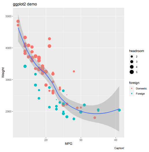
You can get much more complex with the figure, like specifying colors by foreign status, specifying dot size by headroom size, adding a loess curve with 95% CI, and adding some labels. You can swap out the “rcall: e <- ggplot(…)" bit above for the following. Remember to end every non-final line with the three forward slashes.
Let’s make a figure in ggstatsplot using Stata and Rcall
Here’s some demo code to make a figure with ggstatsplot (which is very awesome and you should check it out). If your ggstatsplot command extends across multiple lines, make sure to end each line (except the final line) with the three forward slash (“///”) line break notation that is used by Stata.
// load sysuse auto dataset
sysuse auto, clear
// set up rcall, clean session and load necessary packages
rcall clear // starts with a new instance of R
rcall: library(ggstatsplot) // load the ggstatsplot library
rcall: library(ggplot2) // need ggplot2 to save the png
// move Stata's auto dataset over to R and prove it's there.
rcall: data<- st.data() // move auto dataset to r
rcall: names(data) // prove that you can see the variables.
rcall: head(data, n=10) // now look at the first 10 rows of the data in R
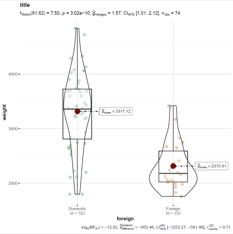
// let's make a violin plot using ggstatsplot
rcall: f <- ggbetweenstats( data = data, x=foreign, y=weight, title="title")
rcall: ggsave("ggstatsplottest.png", plot=f)
// figure out where that PNG is saved:
rcall: getwd()
If you check your working directory (it was my “Documents” folder in Windows), you’ll find this figure as a PNG:
You can automate the output of ggstatsplot figures by editing the ggplot2 components that make it up. You’d insert the following into the ggstats plot code in the parentheses following “ggbetweenstats” to make the y scale on a log axis, for example:
Quick do file to automate R-Stata integration and make ggplot2 or ggstatsplot figures
I made a do file that simplifies the setup of Rcall. Specifically, it 1. Sets R’s working directory to match your current Stata working directory, 2. Starts with a fresh R install, 3. Loads your current Stata dataset in R, and 3. Loads ggplot2 and ggstatsplot in R.
To use, just load your data, run a “do” command followed by the URL to my do file, then run whatever ggplot2 or ggstatsplots commands you want.This assumes you have installed R, the required packages, and Rcall (see very top of this page). If you get an error, try using this alternative version of the do file that doesn’t try to match Stata and R’s working directory.
Example code:
// Step 1: open dataset
sysuse auto, clear
// Step 2: run the do file, hosted on my UVM directory:
do https://www.uvm.edu/~tbplante/rcall_ggplot2_ggstatsplot_setup_v1_0.do
// if errors with above, use this do file instead:
// do https://www.uvm.edu/~tbplante/rcall_ggplot2_ggstatsplot_setup_alt_v1_0.do
// Step 3: run whatever ggplot2 or ggstatsplot code you want:
rcall: e<- ggplot(data, aes(x=mpg, y=weight)) + ///
	geom_point(aes(col=foreign, size=headroom)) + ///
	geom_smooth(method="loess") +   ///
	labs(title="ggplot2 demo", x="MPG", y="Weight", caption="Caption!")
rcall: ggsave("ggtest.png", plot=e)
Example 2: Using “comorbidity” R package in Stata with Rcall to estimate Charlson comorbidity index or Elixhauser comorbidity score
Here’s some semicolon delimited Stata code to run from a Stata do file apply the Charlson comorbidity index to some Stata data.
webuse australia10, clear // load a default stata dataset with an ICD10 variable
gen id=_n // make an ID by row as there's no ID variable in this dataset

#delimit ;
rcall clear ;
rcall: library(comorbidity) ; // load comorbidity package
rcall: data<- st.data() ; // move data to r
rcall: names(data) ; // look at data
rcall: head(data, n=10) ; // look at rows
rcall: charlston <- comorbidity(x=data, id="id", code = "cause",
		map = "charlson_icd10_quan", assign0 = FALSE) ;
rcall: score(x=charlston, weights = "charlson", assign0=FALSE) ;
rcall: mergeddata <- merge(data, charlston, by="id") ; // merge the original & new charlson data
rcall: head(mergeddata, n=10) ; // look at rows
rcall: st.load(mergeddata) ; // kick the merged data back to stata
#delimit cr
Example 3: Predicting race by last name and sex by first name using the ‘predictrace’ package
Here’s how to use this package in Stata using Rcall. There is a lot of nuance in this package so make sure to read the paper and the github page.
In R, type:
install.packages(predictrace)
Then in Stata, write a do file that generates a variable called “lastnames” that is lower case last names (for race matching) and “firstnames” that is lowercase first names (for sex matching). Below is the code to estimate race by last name (first batch of code) and then sex by first name (second batch of code). This is semicolon delimited.
Estimating race by last name
(Note: this considers “Hispanic” to be a race and not an ethnicity…)
// Clear memory, input dataset of first and last names.
// Here, I'm formatting the strings so they are up to 100 characters
// in length so they don't get clipped (str100).
// If I specified str5 then "Flintstone" would be "Flint".
clear all
input str100 firstname str100 lastname
"Jacob" "Peralta"
"Rosa" "Diaz"
"Terrence" "Jeffords"
"Amy" "Santiago"
"Charles" "Boyle"
"Regina" "Linetti"
"Raymond" "Holt"
"Michael" "Hitchcock"
"Norman" "Scully"
end

compress firstname // optional, shortens string format from 100 char to the minimum length
compress lastname // optional, shortens string format from 100 char to the minimum length

// now replace all names with their lower case variant:
replace firstname = lower(firstname) // first name isn't used here fyi
replace lastname = lower(lastname)

#delimit ;
rcall clear ;
rcall: library(predictrace) ; // load predictrace
rcall: data<- st.data() ; // move data to r
rcall: names(data) ; // look at names of data
rcall: head(data, n=10) ; // look at first 10 rows
rcall: lastnamevector <-data[, "lastname"] ; // make vector from lastname column
rcall: data = merge(data, predict_race(lastnamevector), by.x = 'lastname', by.y = 'name', sort = FALSE) ;
rcall: head(data, n=10) ; // look at rows
rcall: st.load(data) ; // kick the merged data back to stata
#delimit cr
Estimating sex by first name
// Clear memory, input dataset of first and last names.
// Here, I'm formatting the strings so they are up to 100 characters
// in length so they don't get clipped (str100).
// If I specified str5 then "Flintstone" would be "Flint".
clear all
input str100 firstname str100 lastname
"Jacob" "Peralta"
"Rosa" "Diaz"
"Terrence" "Jeffords"
"Amy" "Santiago"
"Charles" "Boyle"
"Regina" "Linetti"
"Raymond" "Holt"
"Michael" "Hitchcock"
"Norman" "Scully"
end

compress firstname // optional, shortens string format from 100 char to the minimum length
compress lastname // optional, shortens string format from 100 char to the minimum length

// now replace all names with their lower case variant:
replace firstname = lower(firstname)
replace lastname = lower(lastname) // last name isn't used here fyi

#delimit ;
rcall clear ;
rcall: library(predictrace) ; // load predictrace
rcall: data<- st.data() ; // move data to r
rcall: names(data) ; // look at names of data
rcall: head(data, n=10) ; // look at first 10 rows
rcall: firstnamevector <-data[, "firstname"] ; // make vector from firstname column
rcall: data = merge(data, predict_gender(firstnamevector), by.x = 'firstname', by.y = 'name', sort = FALSE) ;
rcall: head(data, n=10) ; // look at rows
rcall: st.load(data) ; // kick the merged data back to stata
#delimit cr
Special thanks to Katherine Wilkinson for her R brilliance in debugging this.
Example 4: Making a heatplot with lattice/levelplot
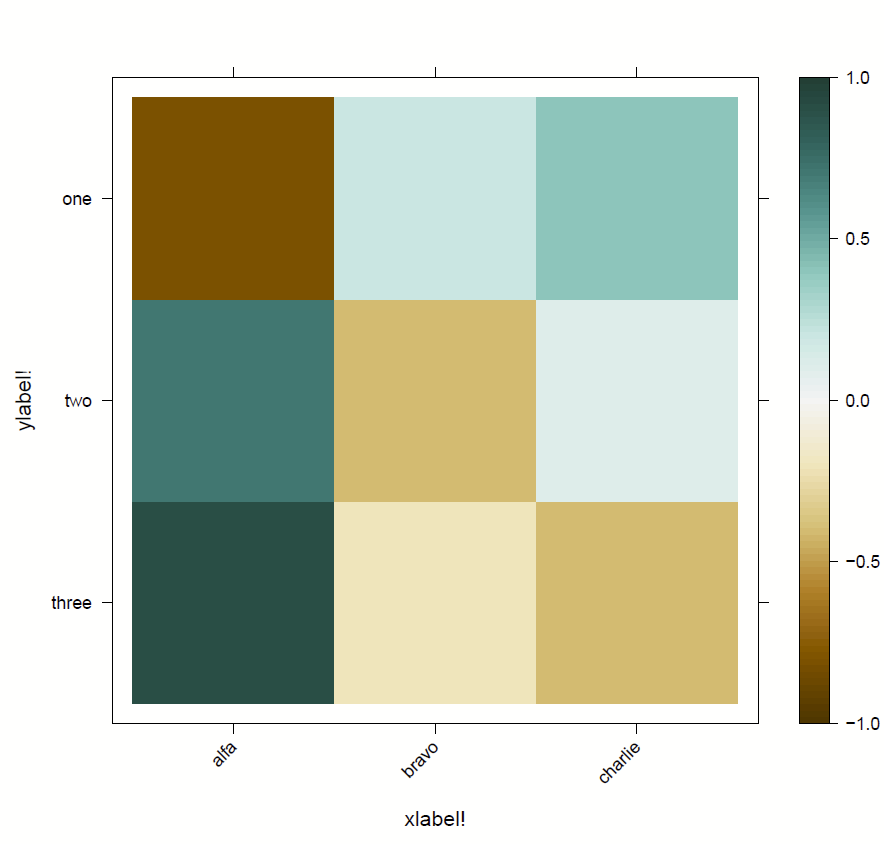
I wanted to make a heatplot ranging from -1 to +1 and wanted the negatives to be a different color from the positives, and have them turn more muted as they get to zero. I couldn’t quite figure out how to do this with the –twoway contour– or –plotmatrix– commands. It was pretty simple to do these in R, just needed to use the RColorBrewer package, specifying “BrBG” as the palette. I used the “lattice” package and its “levelplot” command as described in this post.
In R, install the lattice and RColorBrewer packages (lattice was already installed on my R desktop):
Now in Stata, input the data you’re interested in rendering in order of columns left to right then each column. Then, kick it to R, load the necessary libraries, grab your colorbrewer scheme of choice, label the axes, and then use the “levelplot” to render this. It will save a PDF in your R working directory. I couldn’t for the life of me figure out how to save it as a PNG but there was diminishing returns on figuring that out.
clear all
input x y z
-0.8 0.2 0.4
0.7 -0.4 0.1
0.9 -0.2 -0.4
end

#delimit ;
rcall clear ;
rcall: data<- st.data() ; // move data to r
rcall: names(data) ; // look at names of data
rcall: head(data, n=10) ; // look at first 10 rows
rcall: library(lattice) ; // load packages
rcall: library(RColorBrewer) ;
rcall: colors <- colorRampPalette(brewer.pal(16, "BrBG")) ; // get colors
rcall: colnames(data) <-c("alfa", "bravo", "charlie") ; //names of columns and rows
rcall: rownames(data) <-c("one", "two", "three") ;
rcall: levelplot(
		t(data[c(nrow(data):1) , ]),
		col.regions=colors,
		xlab="xlabel!",
		ylab="ylabel!",
		at=seq(min(-1), max(1), length.out=100),
		scales=list(y=list(rot=0), x=list(rot=45))
	) ; // pull data, apply colors & labels, set color axis range, rotate labels
rcall: getwd() ; // figure out where that PDF is saved:
#delimit cr