Julia for Stata users 2 – Fundamentals of loading, merging, and viewing data

(See the part 1 post here.)

Viewing and changing your working directory

One step will be changing your working directory to the place where you actually want to be working. See your current working directory with “pwd()“. Note: if you get a message saying “pwd (generic function with 1 method)”, you entered “pwd” and not “pwd()”.

Anyway, here’s what I see:

What’s up with the double slashes in Windows directories? Windows is unique among OSes in that it uses backslashes (\) and not forward slashes (/) in its file structure. It turns out that the backward slash is also special character in coding so you have to do two slashes for “normal” slashes as a translation in a lot of coding programs (details here). If you want to change your directory in Windows, you’ll need to deal with single to double backslashes conversion by either (1) adding a second backslash everywhere it shows up in a directory, or (2) declare the string to be raw as is described here. See more on the second, easier option below.

You can change the directory in Julia with “cd([your directory])“. In Windows explorer, you can copy the path by right-clicking on the desired folder and clicking “copy as path”.
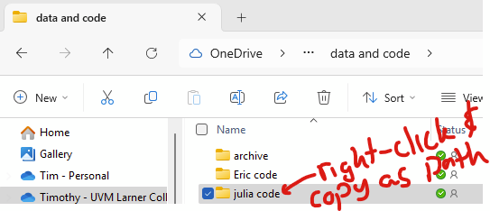
So, to change your directory in windows, you need to deal with how Julia handles backslashes. Adding “raw” before the string of the directory is simpler. The following two are equivalent:

cd("C:\\Users\\USER\\julia code")
cd(raw"C:\Users\USER\julia code")

The second allows you to simply paste the directory from Windows Explorer. So, use raw before your directory string! I don’t know if people will have this problem with other operating systems, I’m guessing not.

You can view the contents of your working directory (e.g., like “ls” or “dir”) with “readdir()“. In this example, I have already used cd() to change my pwd() to the folder that has a Julia script in it:

Hey! It’s my “count to a billion” code from part 1. Since it’s in my current directory, I can load it and run it using the include() command as follows:

include("test.jl")
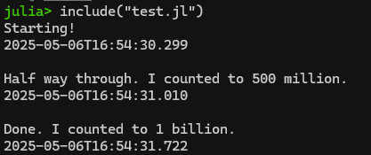
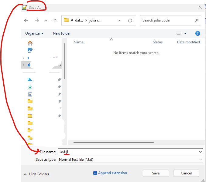
This is actually quite a helpful command if you are writing your script in Notepad++ like we covered in Part 1. Rather than copying/pasting the contents of your script from Notepad++ into Julia/REPL, you can simply do your editing in Notepad++, save the updated script, and then re-run it using include(filename.jl)! A bit less clunky.

Importing files from other statistical packages (SAS’s sas7bdat, Stata’s .dta) using TidierFiles

As discussed in part 1, Tidier is a meta-package that includes a ton of sub-packages in an attempt to create Tidyverse in Julia. One of Tidier’s included packages is the TidierFiles package, which reads and writes all sorts of stuff. Note: You load all Tidier packages, including TidierFiles, when you load Tidier itself. TidierFiles uses Julia’s revered DataFrame package, FYI. You’ll see “df” to name imported data sitting in a dataframe.

Step 1: Installing Tidier (and with it, TidierFiles) and DataFrame

In the package manager (hit “]” to enter), type “add Tidier”. After they install, hit backspace to get back to Julia’s REPL. Alternatively, you can run the following in the REPL or in a script to install Tidier:

using Pkg # need to remember to load Pkg itself!!
Pkg.add("Tidier") # This loads lots, including TiderFiles and DataFrame
Pkg.status() # see that it installed. 
using Tidier # load tidier
# type ? and "Tidier" to see all of the packages that come with it.
# type ? and "Tidier.TidierFiles" to read about that specific package.

Step 2: Importing SAS, Stata, CSV and other files

Importing SAS: Now let’s download the airline.sas7bdat dataset from here: https://www.principlesofeconometrics.com/sas.htm — save it to your pwd(). The following command (1) uses Tidier’s TidierFiles to import the airline.sas7bdat as a DataFrame called “df” then (2) shows that it loaded correctly using varinfo().

Note: You can opt to use “read_file” instead of “read_sas” and let TidierFiles figure out what type of file it is. In 2025, this gives an error if you are trying to automate the download using a string, so better to use the “read_sas” command here.

using Tidier # this loads TidierFiles
# set pwd() with cd(), confirm you did it correctly with pwd(), then read the pwd() contents with readdir()
cd(raw"C:\YOUR DIRECTORY")
pwd()
readdir() # the airline file should be in the pwd()
# the following saves the sas file as a dataframe called "df1"
df1 = read_sas("airline.sas7bdat") 
# see that it loaded as a dataframe: 
varinfo()
# fin

In theory, you should also be able to load the above file directly from the web, but I’m getting an IO error doing that. I’ll come back and try to debug later. This should be the correct code, I’m not sure why it’s not working.

using Tidier
# set pwd() with cd(), confirm you did it correctly with pwd(), then read the pwd() contents with readdir()
cd(raw"C:\YOUR DIRECTORY")
pwd()
readdir()
df2 = read_sas("http://www.principlesofeconometrics.com/sas/airline.sas7bdat")
# see that it loaded as a dataframe: 
varinfo()
# fin

Alternatively, you can instead use Julia to download a file to your pwd() in a script. Let’s say you want to download the andy.sas7bdat file and save it to the pwd(). the Downloads package can help with that. Install it with “]” and “add Downloads” or “using Pkg” and “Pkg.add(“Downloads”)”.

using Tidier
using Downloads
# set pwd() with cd(), confirm you did it correctly with pwd(), then read the pwd() contents with readdir()
cd(raw"C:\YOUR DIRECTORY")
pwd()
readdir()

# specify the URL
url = "http://www.principlesofeconometrics.com/sas/andy.sas7bdat"

# Specify the destination, but need to explicitly name the file
# so grab the filename from the end of the URL and list it
# along with the pwd using the joinpath command
filename = split(url,"/") |> last 
dest = joinpath(pwd(), filename)
Downloads.download(url, dest)

# see that the file is downloaded in your pwd()
readdir()

# Now use the above script to import the andy file, using the
# captured filename string to automate the import
df3 = read_sas(filename)
# see that it loaded as a dataframe: 
varinfo()
# fin

Importing Stata: This is essentially identical to importing a SAS file, but use the “read_dta” command in place of “read_sas”. If you had the auto.dta file in your working directory, this is how you’d import it.

using Tidier
using Downloads
# set pwd() with cd(), confirm you did it correctly with pwd(), then read the pwd() contents with readdir()
cd(raw"C:\YOUR DIRECTORY")
pwd()
readdir()
df4 = read_dta("auto.dta")
# see that it loaded as a dataframe: 
varinfo()
# fin

Here’s how that’d look using the auto.dta file from Stata’s website (https://www.stata-press.com/data/r17/r.html):

using Tidier
using Downloads
# set pwd() with cd(), confirm you did it correctly with pwd(), then read the pwd() contents with readdir()
cd(raw"C:\YOUR DIRECTORY")
pwd()
readdir()

# specify the URL
url = "https://www.stata-press.com/data/r17/auto.dta"

# Specify the destination, but need to explicitly name the file
# so grab the filename from the end of the URL and list it
# along with the pwd using the joinpath command
filename = split(url,"/") |> last 
dest = joinpath(pwd(), filename)
Downloads.download(url, dest)

# see that the file is downloaded in your pwd()
readdir()
# now import that file as a dataframe:
df5 = read_dta(filename)
# see that it loaded as a dataframe: 
varinfo()
# fin

Here you go!

Importing CSV and other filetypes – TidierFiles will import “csv”, “tsv”, “xlsx”, “delim”, “table”, “fwf”, “sav”, “sas”, “dta”, “arrow”, “parquet”, “rdata”, “rds, and Google sheets, you just need to select the correct command to do so (see details here) to replace “read_sas” and “read_dta” above.

Step 3: Merging DataFrames together

We’ll use NHANES data (saved as sas7bdat) and merge on SEQN, aka a unique identifier. The following script downloads the DEMO file and a cholesterol file, and saves them in DataFrames called df_demo and df_trigly

using Tidier
using Downloads
# set pwd() with cd(), confirm you did it correctly with pwd(), then read the pwd() contents with readdir()
cd(raw"C:\YOUR DIRECTORY")
pwd()
readdir()

# Demo file
url = "https://wwwn.cdc.gov/Nchs/Data/Nhanes/Public/2013/DataFiles/DEMO_H.xpt"
filename = split(url, "/") |> last 
dest = joinpath(pwd(), filename)
Downloads.download(url, dest)
readdir()
df_demo=read_sas(filename)


# Cholesterol file
url = "https://wwwn.cdc.gov/Nchs/Data/Nhanes/Public/2013/DataFiles/TRIGLY_H.xpt"
filename = split(url, "/") |> last 
dest = joinpath(pwd(), filename)
Downloads.download(url, dest)
readdir()
df_chol=read_sas(filename)


# look at dataframes and strings loaded:
varinfo()
# fin

Now, let’s merge/join the df_demo and df_chol dataframes together and save it as a dataframe called df_merge. This will use TidierData’s join function, you can read about here. There are a bunch of different joins, we’ll be doing a full_join which will preserve all rows without dropping any for missing. Read about joins (“merge”) here. Of note, the join command as implemented in TidierData will infer the matching variable based upon identical columns in the two datasets. Continuing with the prior script:

df_merge = @full_join(df_demo, df_chol)

Combined code:

using Tidier
using Downloads
# set pwd() with cd(), confirm you did it correctly with pwd(), then read the pwd() contents with readdir()
cd(raw"C:\YOUR DIRECTORY")
pwd()
readdir()

# Demo file
url = "https://wwwn.cdc.gov/Nchs/Data/Nhanes/Public/2013/DataFiles/DEMO_H.xpt"
filename = split(url, "/") |> last 
dest = joinpath(pwd(), filename)
Downloads.download(url, dest)
readdir()
df_demo=read_sas(filename)


# Cholesterol file
url = "https://wwwn.cdc.gov/Nchs/Data/Nhanes/Public/2013/DataFiles/TRIGLY_H.xpt"
filename = split(url, "/") |> last 
dest = joinpath(pwd(), filename)
Downloads.download(url, dest)
readdir()
df_chol=read_sas(filename)

# join/merge datasets, save as "df_merge" dataframe
df_merge = @full_join(df_demo, df_chol)
# look at dataframes that are there:
varinfo()
# fin

Exporting data

You can export your work using TidierData, just use “write_sas”, “write_dta”, “write_csv” or whatever you want. Details are here. For example, you can append the following to the end of the prior code and save the df_merge dataframe as a CSV file in your pwd(), including the column names as the first row.:

write_csv(df_merge, "NHANES_merged.csv", col_names=true)
# fin

Saving your work in Julia’s JLD2 format and then later loading it

The JLD2 file format seems to be designed to be compatible with future changes in Julia. See details here. Install it in the Pkg interface (hit “]”) then “add JLD2” or “using Pkg” and “Pkg.add(“JLD2″)”. You can save things in your memory (type “varinfo()” to see what’s loaded). For example, you can save the df_merge from 2 sections above with:

using JLD2
# set pwd() with cd(), confirm you did it correctly with pwd(), then read the pwd() contents with readdir()
cd(raw"C:\YOUR DIRECTORY")
pwd()
readdir()
@save "mydataframe.jld2" df_merge
# look at files in pwd()
readdir()
# fin

I haven’t quite found an elegant way to reload JLD2 with Tidier, it instead uses DataFrames (which is actually included in Tidier but doesn’t correctly work with this). You’ll need to separately install DataFrames in the Pkg interface (hit “]” and type “add DataFrames” or in REML type “using Pkg” and “Pkg.add(“DataFrames”)

# close and reopen Julia, load JLD2 and DataFrames
using JLD2
using DataFrames
# set pwd() with cd(), confirm you did it correctly with pwd(), then read the pwd() contents with readdir()
cd(raw"C:\YOUR DIRECTORY")
pwd()
readdir()
# load the dataframe as df_merge.
@load "mydataframe.jld2" df_merge
# look at dataframes and strings loaded:
varinfo()
# fin

Viewing your data in the browser

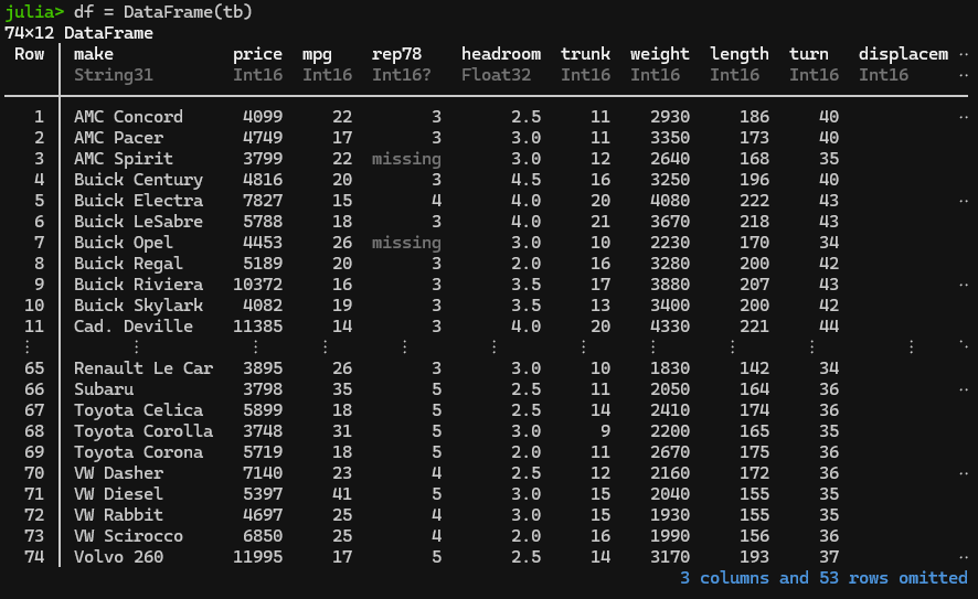
One great Stata feature is “browse”, allowing you to look at all of the data. The “BrowseTables” package allows you to do something similar in Julia’s interface and (more importantly) a browser window. We will demonstrate this using the merged NHANES dataset above.

Jump to the pkg interface (hit “]”) and type “add BrowseTables” or add in REPL with “using Pkg” and “Pkg.add(“BrowseTables”) then the following:

using BrowseTables
# view 'whatever fits' in the julia terminal:
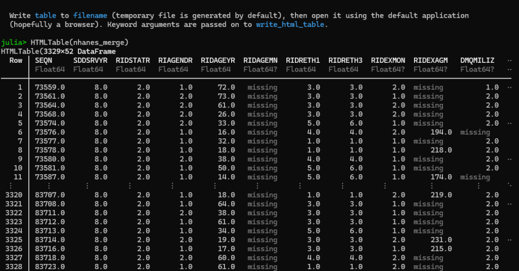
HTMLTable(df_merge)

# open up the nhanes_merge example from above in a browser:
open_html_table(df_merge)
# fin

The first command, HTMLTable(df_merge), will show output in the Julia browser, truncating the columns and rows so that it fits like such:
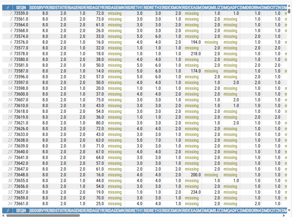
The second command, open_html_table(df_merge), will open the entire dataset in your default browser, like so:
Stata’s ‘browse’ feature is nice in that it allows you to browse subsets of data, e.g., ‘browse if sex==”M”‘ would show data for just males. I’ll play around with this a bit more and see if there’s a simple way to subset the rendered tables to just a sample of the data.

Julia for Stata users: Part 1 – getting set up

I’m a big fan of Stata because of its simplicity and excellent documentation. I have a lot of colleagues that use R and I see why they like it, but I’m not a fan of the R syntax. I’ve played with Python and liked the syntax quite a bit but found simply installing Python and its packages to be really annoying on Windows.

The Julia language seems to have some of the nice features of R (e.g., arrays start at 1, Tidyverse-like packages, ggplot2 was rewritten in Julia) and syntax similar to Python. Julia seems to have a unique(?) feature called “broadcasting” (with shorthand being just a dot or “.”) that allows you to run commands by row. The help files seem okay, though pretty brief. Julia users aren’t typically huge jerks on online forums. I’ve read online that the speed of Julia is very attractive to R users (but I do epidemiology work in ‘relatively’ small datasets, e.g., <1 million observations, so speed of my statistical packages doesn't really make a difference in my analyses). It is similar to Stata in that missing values are treated as positive infinity. Unlike Stata, it'll use all available CPU cores in the base version (Stata only uses a single core unless you pay for a more expensive version). Finally, Julia seems to be pretty well-developed for AI/ML (as are R and Python), which is something that Stata leaves to be desired.

My main reservation about Julia is that it’s relatively new since it was only started ~13 years ago (it’s currently 2025) so it’s not going to have every package or instructional post under the sun. It’s old enough that I expect the language to be reasonably well-developed though. I’m also not a huge fan of capital letters in coding since I’m used to Stata and everything in Stata is lower case. That’s DEFINITELY not the case in Julia, and Julia is not at all forgiving if you type “using pkg” instead of “using Pkg”. But I thought I’d give it a go!

To the point of Tidyverse, my perspective is that much of the rise of R’s popularity is in the development and uptake of Tidyverse. Tidyverse is a meta-package that brings together a bunch of individual packages that simplify data analysis. Core to Tidyverse is the concept of “tidy data”, meaning that:

  1. Each variable is a column; each column is a variable.
  2. Each observation is a row; each row is an observation.
  3. Each value is a cell; each cell is a single value.

…for Stata users, that should sound familiar since it’s the exact data structure that Stata uses. Only columns are called “variables” and rows are called “observations”. Conceptually, tidy data and the Tidyverse makes R run like Stata. For Julia, there is an implementation of the Tidyverse called Tidier that started ~2 years ago (it’s 2025). Like Tidyverse, Tidier is a meta-package including lots of subpackages:

  • TidierData – For data manipulation, like R’s dplyr and tidyr
  • TidierPlots – For figures, an R implementation of ggplot2
  • TidierFiles – For reading and writing different filetypes, like R’s haven and readr
  • TidierCats– For managing categorical data, like forcats
  • TidierDates – For managing dates/time, like lubridate
  • TidierStrings – For managing strings, like stringr
  • …and a few others

Unlike Stata, Julia is intended to have an infinite amount of “datasets” open at once, some can just be a single string, some can be a vector of data, some can be a full dataframe. However, Tidier is designed to function on only a single dataframe so if needing to include something from a “dataset” outside of the current dataframe, you need to precede the Tidier command with @eval and use a dollar sign in front of whatever the non-current-dataframe thing is. This is called interpolating, and details are here.

There aren’t many drawbacks to using Tidier that I can find, other than it being pretty new and it taking about 15-30 seconds to load the first time you load (“using”) it in a Julia session.

This series of posts documents my foray into the Julia language, being an epidemiology-focused user of Stata on Windows, with an emphasis on using Tidier. Note that Mac and Linux users can probably follow along without any problems, though the installation might be slightly different.

Things that annoy me about Julia

As I’m putting these pages together, I’m coming back to document what annoys me about Julia. Here’s an incomplete list:

  • Lack of forgiveness with capitalization. I’m sorry that I typed “pkg” instead of “Pkg”. Cmon though, can you let it slide? Or at least let me know that it’s a capitalization problem?
  • Pkg isn’t auto-loaded with Julia. C’mon…
  • Strings with backslashes or dollarsigns ($) and probably other characters will confuse Julia. The simple workaround is to smush ‘raw’ before the opening quote of these strings, e.g., raw”$50,000″
  • Sorting functions appear to sort by capital letters first, so “Zebra” would be sorted to be above “apple”. The workaround is to generate a lowercase column and sort on that. It’s clunky.
  • Slowness with loading packages the first time (in 2025). Tidier takes 30 seconds to load, and that’s not unique to Tidier. Yes, Julia is reported to be faster than R, but it doesn’t seem zippy when you are loading things.
  • Needing to manually load packages before using them. It would be nice for Julia to load packages on the fly when called the first time.
  • No way to ‘reset’ Julia like the ‘clear all’ command does to Stata. The current workaround is to close down Julia and open it up fresh.
  • No ‘cheat sheets’ for Julia packages (in 2025) like the awesome ones that have been written for Stata and R. There is a nice ‘general’ Julia cheat sheet though.

Installing Julia on Windows 11

Installing it from the command line prompt is incredibly simple. It automatically sets the PATH and whatnot. Steps: Hit win key + R to open the run prompt, then type “cmd” without quotes to open the command line in Windows (or just hit the start button and type “cmd” and click on “command prompt”), and drop the prompt listed here: https://julialang.org/install/

You can also manually install from the Julia Downloads page, but I would honestly follow the guidance on the install page above and do the command line prompt install. But here’s the Downloads page in case you need it: https://julialang.org/downloads/

The Julia download page also lists a portable version of Julia that you can run off a thumbdrive or as a folder on your desktop without needing to formally install it!: https://julialang.org/downloads/ (I’d get the 64 bit version, unlikely that you’ll run into a 32 bit windows PC these days. You can check your Windows version in cmd by entering “wmic os get osarchitecture”.) You just unzip the folder where you want it. You can run Julia by clicking “bin\julia.exe”. It takes about 30 seconds to open, but it works!

Running Julia on Windows 11

There are a few ways to run Julia. Since I’m just starting out, I’ll be using Option 1, which is a lot simpler.

Option 1 – Write Julia’s *.jl scripts in Notepad++ and run by copying/pasting them into Julia running in the Windows Terminal — aka the ‘low tech’ way

I’m a HUGE fan of Notepad++ as a text editor, and it works very well to write Julia scripts. (Notepad++ is for Windows only. If you are on MacOS or Linux, you might want to try Sublime Text Editor instead.) You’ll want to get the markup to reflect the Julia language. Steps:

  1. Download and install Notepad++ (get the 64-bit version, aka x64)
  2. Add Julia markup to Notepad++ as follows:
    • Download the XML file here: https://github.com/JuliaEditorSupport/julia-NotepadPlusPlus (click the XML file then click the “download as raw” button that’s a couple over from the “raw” button).
    • In Notepad++, click Language –> User defined language –> Define your language… and then import the XML file.
  3. To test it out, select Julia markup from the language list (Language –> way below the alphabetized list click “Julia”).

FYI, there is a portable version of Notepad++, so you can install it from your thumbdrive or local folder without having to install it. This would match a portable version of Julia. Details: https://portableapps.com/apps/development/notepadpp_portable

Now make a new script and save it as a Julia script file with the extension “*.jl” (that’s a J and an L). When you save with that file extension, Notepad++ automatically knows it’s for the Julia language and will apply your downloaded Julia markup.

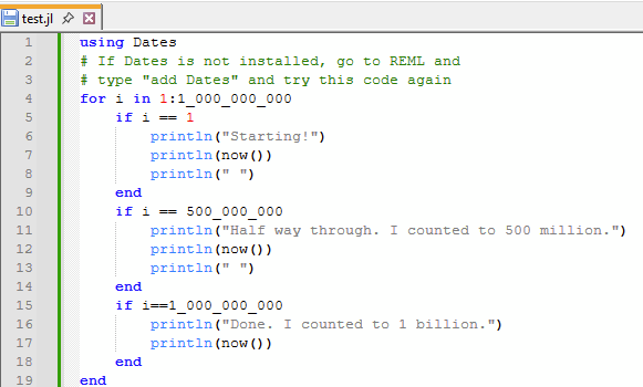
Here’s an example program. I adapted an example counter to 1 billion from section 2.1 of this great Julia Primer from Bartlomiej Lukaszuk: Romeo and Julia, where Romeo is Basic Statistics. Note that you can add an underline in large numbers to make them a bit more readable, so “1000000000” in Julia is equivalent to “1_000_000_000”.

using Dates
# If Dates is not installed, go to the pkg interface ("]") and 
# type "add Dates" and try this code again
for i in 1:1_000_000_000
	if i == 1
		println("Starting!")
		println(now())
		println(" ")
	end
	if i == 500_000_000
		println("Half way through. I counted to 500 million.")
		println(now())
		println(" ")
	end
	if i==1_000_000_000
		println("Done. I counted to 1 billion.")
		println(now())
	end
end
# fin

If you copy and paste that into a *.jl file, you’ll see colored markup.

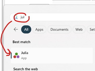
Double clicking the Julia link on the start menu opens up Julia in Windows Terminal by default (on my computer).

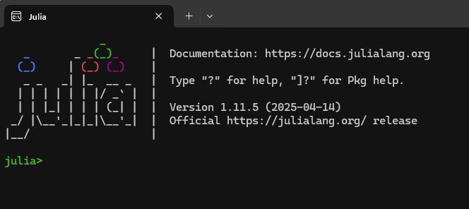
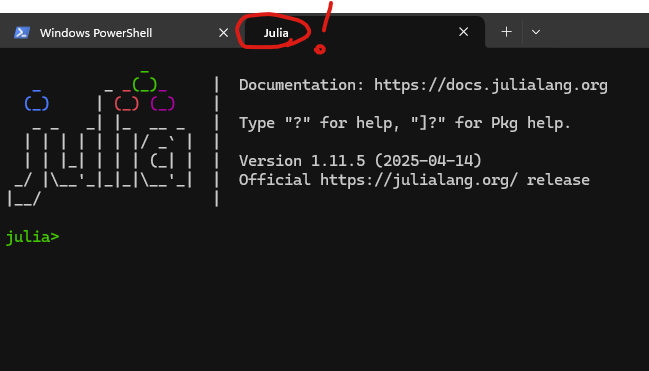
Here’s what Windows Terminal looks like with Julia running:

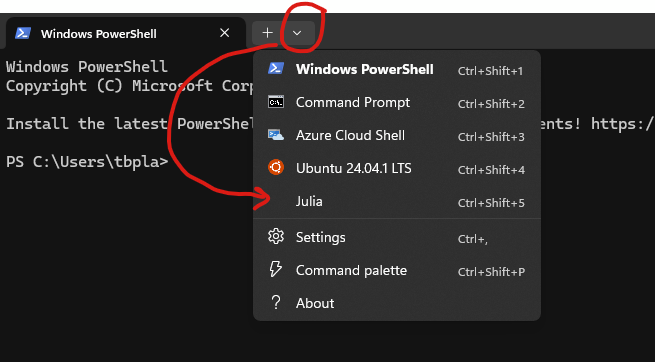
FYI, You can also open Julia from within Windows Terminal, just pop open the run prompt (win key + R) then type “wt” to open up Windows Terminal. It opens up Powershell by default, but there’s a little drop down that allows you to switch to Julia. Neat!

In a couple of seconds, Julia will load:

There are a few modes in the Julia interface to know about that you can read about here:

  • REPL mode (“julia>”) – This is the interface for Julia. Enter in all of your commands here. If you are in another mode, hit backspace to get back to REPL.
  • Help (“help?>”) – Enter a question mark (“?”), you enter the help context. You can query commands by typing the command name here.
    • Note: You need to load any package before accessing the help file btw, so if you type “?” then “Pkg”, you get an error. First, load Pkg with “using Pkg” then “?” then “Pkg”, and you’ll get the help file.
    • Note: You can also find help files for subcommands of packages. For example, after loading Pkg, you can type “Pkg.status()” to get a list of all installed packages. In the help screen (again, hit “?” to access it), type “Pkg.status” to see a help file for Pkg.status(). Similarly, if you want to learn about subpackages within Tidier, you need to list them after a dot, e.g., “Tidier.TidierDates”, or subsubpackages/commands by stringing multiple dots, e.g., “Tidier.TidierDates.difftime”.
    • Hit backspace to go back to REPL.
  • Shell (“shell>”)- Hit the semicolon (“;”) to get to the system shell. I have no idea how accessing the shell is of any value to me for what I’d use Julia for.
    • In Windows, you need to secondarily open Powershell by then typing “powershell” or the command prompt by typing “cmd”.
    • Hit backspace to go back to REPL.
  • Pkg to install/add new packages (“Pkg>”) – Aka installing new programs.
    • Type “add” and the name of the package of interest to install the package. E.g., “add Dates”.
    • Type “status” to see installed packages.
    • Type “update” to update all packages.
    • Hit backspace to go back to REPL.

But how do you run scripts from Notepad++ in Julia’s REPL mode? When you want to run bits of your script, simply copy and paste it into the Julia REPL interface. Note: One little glitch is that when you paste into REPL, the last line doesn’t load until you hit enter, you’ll see it just chilling on the input (e.g., “Julia > end”) when you copy/paste. You can do a workaround by having the last line of your code be a comment that isn’t actually needed to run your code. I’m using “# fin” as my last-line comment because it’s super classy. If you see “# fin” hanging out on the “Julia>” input line in REPL, just delete it before pasting anything else or your first line will follow “# fin” and be interpreted as a comment by Julia.

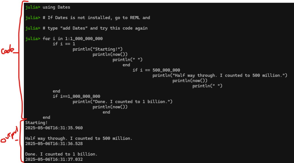
If you copy above and paste the “count to a billion” code from Notepad++ into the Windows Terminal running Julia, you get the following:

Cool! Julia counted to 1 billion in a little over 1 second. WOW THAT’S FAST!

In Part 2, I show an alternative way of running a script you are updating and saving in Notepad++ from within Julia, rather than copying and pasting everything.

Option 2 – Visual Studio Code with the Julia extension, aka the R Studio of Julia

R Studio is the most iconic Integrated Development Environment (IDE) for R. There were a few projects intending to be IDEs for Julia (e.g., Atom and Juno) that have halted development in support of Visual Studio (VS) Code’s Julia extension. VS Code is a general-purpose IDE developed by Microsoft that’s widely used in computer science and is available for all sorts of operating systems, not just Windows. VS Code should not be confused with Visual Studio, which is another IDE that Microsoft makes. The core of VS Code is open source, but the specific VS Code download from Microsoft isn’t.

Despite being a long-time Windows and Office user, I’m really not a fan of Microsoft products. They tend to be bloated and include whatever is trendy in the business world. VS Code is pretty bloat-free but does include a ‘bloaty’ AI assistant. I find VS code to be a bit overwhelming, which is why I like Notepad++.

Downloading VS code:

You can also install VS Code as a portable app, so presumably you can have a portable version of Julia and also a portable version of VS Code both running from a thumbdrive or desktop folder without requiring an install. Details are here: https://code.visualstudio.com/docs/editor/portable

I might one day switch over to VS Code, but for now I’m sticking with Notepad++ and Windows Terminal.

Option 3 – Using Pluto notebooks, aka the Julia equivalent to Jupyter notebooks

Jupyter notebooks are ‘reactive’ notebooks that allow you to write and execute code in a browser, and see results in-line. Jupyter notebooks are great but require Python for their use. Pluto is very similar to Jupyter notebooks except implemented using Julia code alone — no requirement for Python. You can read all about Pluto here.

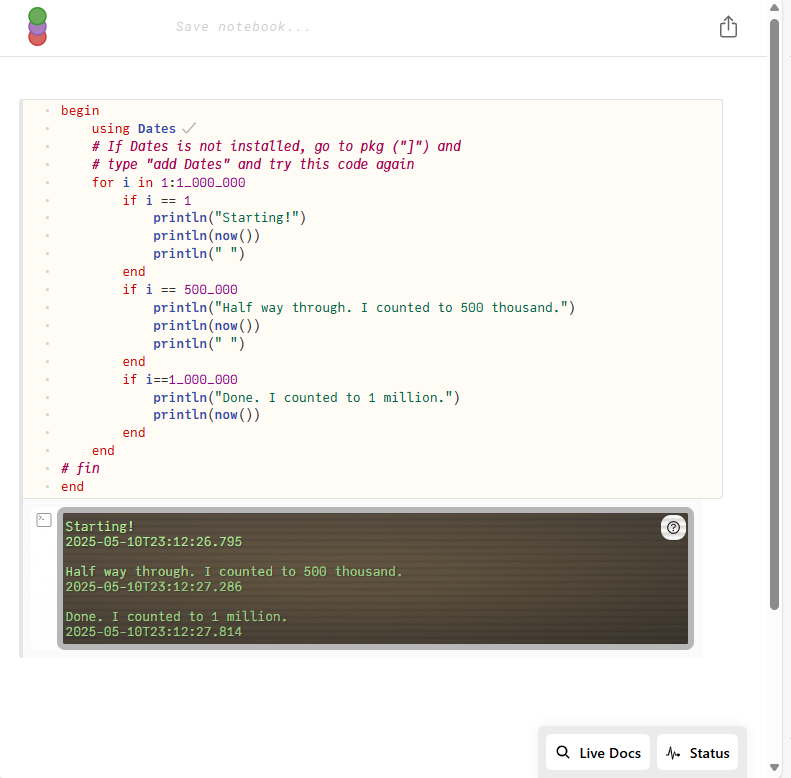
After installing it (‘using Pkg’ and ‘Pkg.add Pluto’), you can run Pluto in a browser by typing ‘Pluto.run()’. You can then run Julia interactively in your browser. If you want to run a block of code all at once (rather than line-by-line), you need to add a “begin” before all of the code and “end” after all of the code and indent what’s in between. Here’s an example of what this looks like, adapting some code for counting to 1 billion from above. (Note that this was taking A REALLY LONG TIME so I made it count to 1 million and not 1 billion.) You’ll see that the code has “begin” and “end” and everything is indented in between. The Julia output shows up below.

Pluto is REALLY COOL and seems user friendly for simple projects. I’m worried about how slow it was compared to the Julia in Windows Terminal. I’ll probably explore it a bit later. For now, I’m sticking with Notepad++ and Julia in Windows Terminal.

Installing packages in Julia

Stata is nice in that it comes with built-in functionality that allows you to do 95% of what you’re trying to do right out of the box. Occasionally you’ll need to install additional ado programs via SSC. Julia (like R) is limited in what it can do out of the box and requires you to install additional packages to add necessary functionality. Julia’s packages are a 2-step process:

  1. Add (ie install) packages of interest.
  2. In your script, call the package with “using”. (There’s also something called “import” that you can read about here that you may want to use instead of “using”. I’m still not entirely sure of the fundamental differences between “import” and “using”, so I’m sticking with “using” for now.)

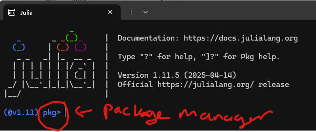
The great thing about Julia is that its package management is VERY simple and baked into its interface. It ships with a package manager “Pkg” (details here) that you can load (“using Pkg”) and then call use to install other packages in a script, or alternatively you can switch over to the package management interface. In the REPL (aka “Julia”), simply hit a closing non-curly bracket (“]”) to open the package manager. Exit the package manager back to REPL by hitting backspace.

Above, you’d just hit the “]” key and see:

Again, just hit backspace to get out of the package manager back into Julia’s REPL interface.

Here’s an example for using Pkg in REPL or a script to download Tidier. Since Tidier is a metapackage with TONS of other packages inside of it, so it’ll take a bit of time to install (“add”), and also will take a bit of time to load (“using”) the first time. Subsequent times that you load (“using”) Tidier will be faster, but it’ll still take ~15 seconds to load each time.

using Pkg # need to make Pkg available to Julia
Pkg.add("Tidier") 
#fin

Example for using the package manager, which you enter by hitting “]” in REPL:

add Tidier

Then hit backspace to exit the package manager back to REPL.

After these packages are installed, you can use them, but you need to make them available to Julia in your script, such as the following (Tidier will take a bit to load the first time, be patient — it’s faster with future loads):

using Tidier
[code that uses Tidier]
# fin

To update packages, use the Pkg.update() functionality, in REPL:

using Pkg
Pkg.update("Tidier")

Or in the Pkg interface (“]”):

update Tidier

Continue reading part 2 here.