
I got to the gap around 10:40 this morning. The temperature was 75 F and the sky was partially filled with clouds. I could feel the humidity rising as yesterday’s rain was evaporated out of the forest.
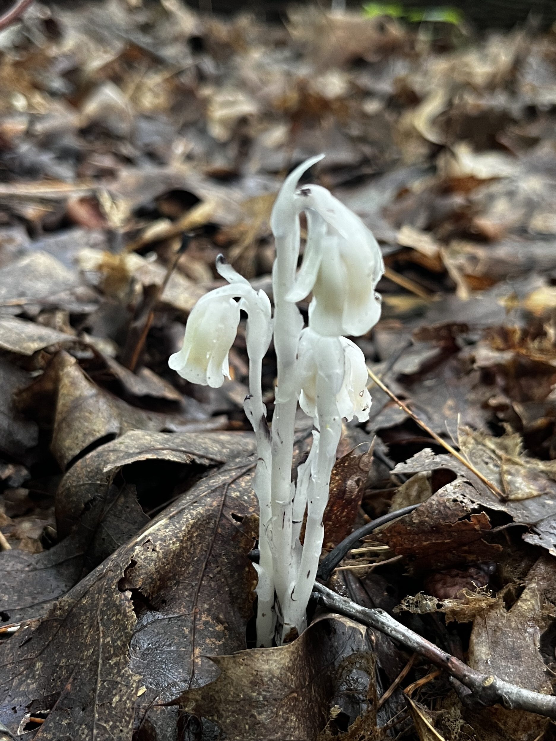
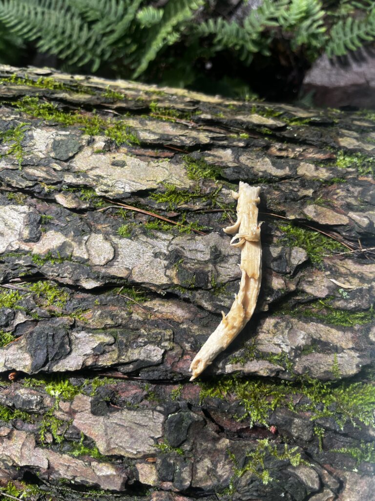
I started my visit today listening to the birds because I noticed it was the first time I really heard any in all of my visits. I pulled out the Merlin bird app and started a recording: black-throated green warbler, red-eyed vireo, black-capped chickadee, cedar waxwing, and eastern wood-pewee. I’m pretty certain I was in the presence of a black-throated green warbler, a black-capped chickadee and a red-eyed vireo. But the rest I was unsure of. I didn’t think I was in the right ecosystem for cedar waxwings and I didn’t hear the infamous “PEE-WEEEE” of the eastern wood-pewee, although it’s entirely possible the Cornell Lab of Ornithology knows better than me. Today I also saw some ghost pipes on my walk to the gap and also evidence of somebody dining on a mushroom. I forgot to take a picture of of the tan, flat-capped mushrooms growing next to this spot, and frankly I wasn’t very interested in them as identifying mushrooms isn’t why I came to the gap today.
I came to the gap today to get answers. I wanted try and quantify the effects of light levels in different parts of the gap on plant growth in those locations. I have been remarking all along about how there is a tremendous amount of plants growing directly in the middle of the gap where there is more sun but up until today, I didn’t have much evidence to prove it – to show there is a difference between in the gap and next to the gap. To test this theory, I devised a simple study to gather data on how many plants (individuals and species) are growing in different parts of the gap and relate that to the amount of canopy cover over that spot.*
*this isn’t really a theory that needs proving (as it’s a common known fact of forest ecology), but I thought it would be fun to apply some hard science to the gap and see if my findings agreed with what is already known.
Hypothesis
Due to higher light levels in the middle of a forest canopy gap, there are more plants growing per square foot than locations adjacent to the gap.
Methods
- I decided to do a sort of seedling/herbaceous study and to use a sampling scheme of 1-sqft. micro-plots at 1ft, 6ft, 11ft, and 16ft along a transect in each cardinal direction emanating from the center of the gap which would give me an idea of how things changed as I got further away from the center of the gap. I marked the center of the gap with a stick to keep it constant throughout sampling. I used a compass and a tape measure to locate and size the 1-sqft. plots.
- At each plot, I counted the number of stems that originated within that plot. For raspberry plants that had both new and old growth stems coming from the same plant, I made sure to only count the plant and not the number of stems coming from that plant. For ground cover that originates from a single plant such as polypody’s, partridgeberry and herb robert, I only counted the number of plants (which basically said if it was present or not).
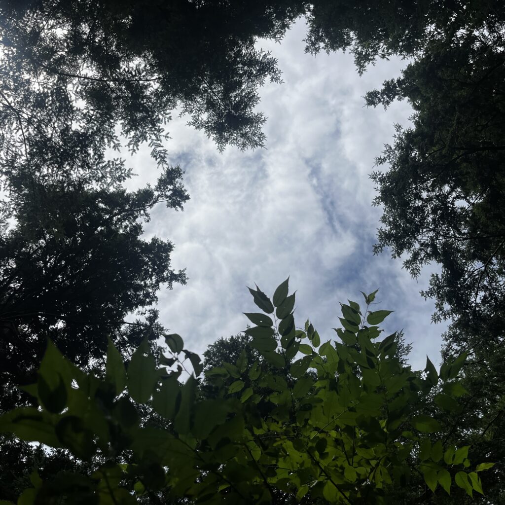
- After collecting the plant data, I took a square-formatted picture looking directly up from the center of the plot. I took the picture from just above the plant growth at that plot which happened to be about 2ft above the ground in most cases.
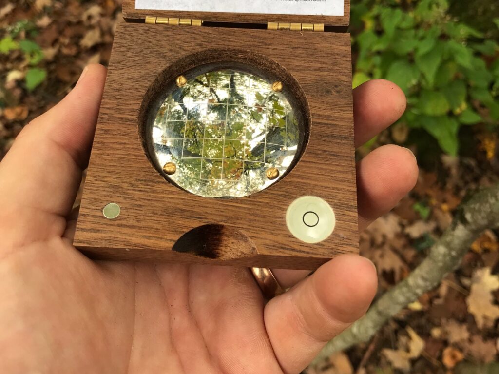
- At home, I wrote a MATLAB script to calculate the percent canopy cover by determining how many of the pixels in the picture were of plants vs sky. In forestry, a canopy densiometer would actually be used in this instance although those instruments are ridiculously expensive for what they are (a curved mirror with a grid of squares). A densiometer is used by holding it flat and counting how many quadrants of each square are showing the sky versus plants. Because densiometers have 24 squares, a total of 96 quadrants and you usually take 4 measurements looking in each direction at each plot, I decided to reduce the resolution of the pictures I took to have a coarser pixel (or quadrant) resolution. A picture of a forest densiometer is shown below.
- Once I had plant and canopy cover data for each plot, I calculated a simple biodiversity metric by dividing the number of species present by the total number of stems counted which results in a value between 0 and 1 (with 1 having the “greatest” biodiversity). I then averaged the values obtained for each distance from the center of the plot and graphed my results.
Results
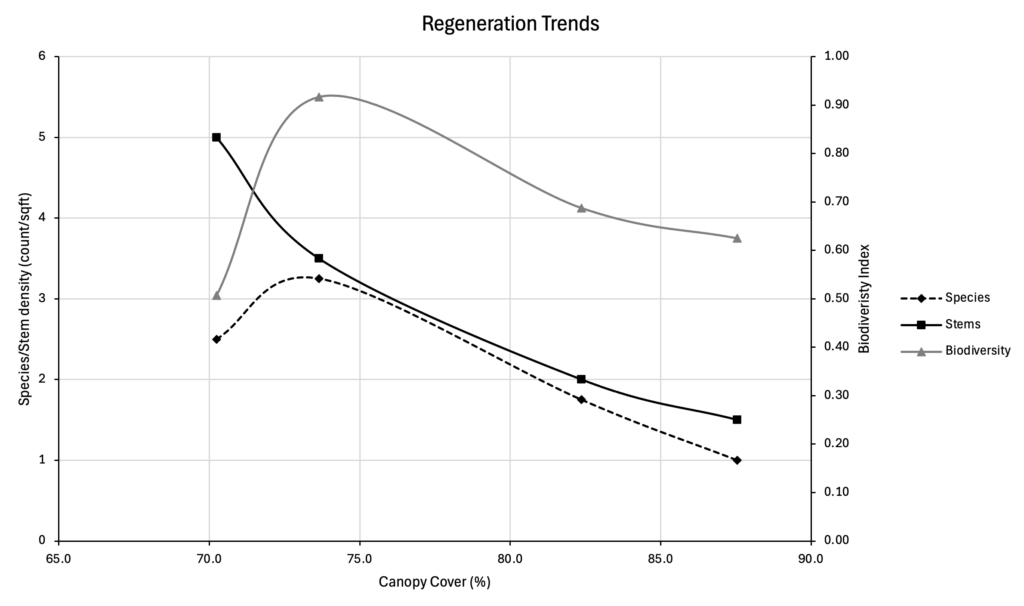
Below is a graph of my results with the number of species, number of individual stems and biodiversity index compared to the percent canopy cover. Note that the x-axis only goes from 65% to 90%. The number of stems per square foot has an inverse relationship as locations with more canopy cover had, on average, less stems growing. However, the number of species per square foot and the biodiversity peaked in the plots 6 feet from the center of the gap and decreased with higher and lower levels of light.
Below is a table showing the values used in the graph above. Note that all values besides the distance from the center of the gap (which was fixed) is an average of the four micro-plots taken at each of the distances. Further below is a table listing the total number of species found between the four plots from each distance along with what those species were. The species are listed the tree species first, then woody shrubs, then herbaceous ground cover.
| Distance (ft) | Canopy Cover (%) | Species density (#/sqft) | Stem density (#/sqft) | Biodiversity index |
| 1 | 70.3 | 2.5 | 5 | 0.51 |
| 6 | 73.7 | 3.25 | 3.5 | 0.92 |
| 11 | 82.4 | 1.75 | 2 | 0.69 |
| 16 | 87.6 | 1 | 1.5 | 0.63 |
| Distance (ft) | Total number of species | Species |
| 1 | 9 | eastern hemlock, ironwood, paper birch, raspberry, red osier dogwood, wild grape, raspberry, partridgeberry, polypody |
| 6 | 10 | green ash, grey birch, sugar maple, pin cherry, striped maple, red osier dogwood, raspberry, clubmoss, herb robert, intermediate wood fern |
| 11 | 7 | ironwood, red maple, chokecherry, wild grape, Canada mayflower, blue-stemmed goldenrod, polypody |
| 16 | 3 | ironwood, red maple, polypody |
Discussion
I think that the results show the story of forest canopy-gap-scale regeneration very well. The results give an answer to my question that higher light levels do lead to higher numbers of plants growing in that particular location. From a resources stand-point, this makes sense as there is physically more sunlight, or photosynthetic opportunity, available per square foot of ground which allows that parcel to support more plant growth.
What I wasn’t expecting was the difference in number of species present at each of the light levels. I had anticipated the center of the gap to have the highest number of species but what the data show suggests a much more nuanced story. I believe the fact that the plots 6 feet from the gap center showed the highest species diversity is because this location is effectively an edge habitat – a place where species from both ends of the spectrum co-habitat. Because there is an intermediate amount of light, the space can support a large set of species that prefer more shade and more sun. It’s also cool how the plots far away from the gap are essentially status-quo plots that show how the forest understory would look without the influence of a canopy gap.
Because I was simply doing counts of stems and species, the data do not say anything about the size of each plant which suggests how long that plant has been growing. It is important to point out that not all of the plants found during this study only were there because of the gap. Species such as sugar maple and eastern hemlock dominate the “advanced regeneration” regime of the forest floor which means grow well in deep shade while the canopy is closed and then are ready to take advantage of higher light levels if/when the canopy is opened. Ironwood, or American hophornbeam, and green ash can also grow under a shaded canopy and was likely there before the gap was created. Pin cherry, on the other hand, germinates from dormant seeds that are present in the soil and begin growing immediately when sunlight hits the ground in high enough levels which suggests they weren’t there before the gap was created. Grey and paper birch also likely weren’t there before the gap as they require higher sunlight levels and were probably blown into the gap by the wind. Striped maple is somewhere between these two camps of shade tolerant and intolerant species and was likely growing before the gap was created and took off once it had enough sunlight.
I am very happy with how my canopy cover MATLAB script works for this process. Using the RGB (red, green, blue) color format, I can easily tweak the script to correctly identify the sky whether it is cloudy or blue skies. To show how the process works from taking the picture to calculating canopy cover, the picture from plot N1 (or the plot on the north transect 1 foot away from the gap center) is shown below in each step of the process. It is not perfect but gives a good estimate of the canopy cover. I think that decreasing the number of pixels isn’t completely necessary (the script produces roughly the same results with pictures of 0.5 pixels/sqin and 20 pixels/sqin) although I think it makes a good approximation for how the same data would be collected with a forest densiometer.


Limitations and Lessons Learned
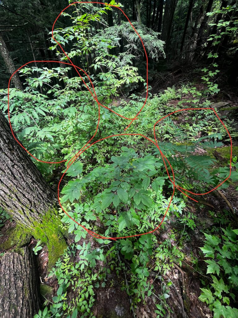
There are a few things I would do differently if I were to do this study again. For one, I would increase the sample size. Having only four plots at each distance leaves some opportunity for variability to skew results. I would also increase the size of the plots to be a square yard or square meter. Although there are a number of species listed as being found in the plots, there were some heavy hitters present in the gap that didn’t get counted in the study. Below is a picture of the gap which shows how much of the space is taken up by a few plants: a staghorn sumac, a green ash, a pin cherry and a BIG elderberry. Additionally, I would make a sample plot boundary with some sticks or pieces of wood in a square that I could place on the ground to have a better idea of what stems are in or out the sample plot.
Closing Remarks about The Gap
Simply put, I’ve had a great time getting to know this little gap of regeneration in Red Rocks park. I loved seeing how the gap changed between visits and also noticing different parts of the site that had stayed the same. I had a great time learning new herbaceous species and bolstering my woody plant ID by getting to identify species I know well but in their often-tricky, seedling form. I am very comfortable with identifying mature woody plant species but seedlings are something that I’ve steered away from in the past so I’m happy to have gotten to learn more about them and gain some experience. I’d like to thank Red Rocks park and my professor Laura Yayac for providing this opportunity to become close with the gap and learn some of its secrets!